WALES Lidar

The water vapour differential absorption lidar WALES. WALES operates at four wave-lengths near 935 nm to measure water-vapor mixing ratio profiles covering the whole atmosphere below the aircraft. The system also contains additional aerosol channels at 532 nm and 1064 nm with depolarization. WALES uses a high-spectral resolution technique, which distinguishes molecular from particle backscatter.

The backscatter product from the HSRL has a resolution of 40 m in the horizontal (corresponding to temporal resolution of 5 Hz and a typical 200 m/s flight speed) and 15m in the vertical, while the water vapor product has approximately 3km horizontal and 250m vertical. The PIs during EUREC4A were Martin Wirth and Heike Gross (DLR).

More information on the instrument can be found in Wirth et al., 2009. If you have questions or if you would like to use the data for a publication, please don’t hesitate to get in contact with the dataset authors as stated in the dataset attributes contact or author.

Note

Due to safety regulations the Lidar can only be operated above 6 km which leads to data gaps in about the first and last 30 minutes of each flight.

import eurec4a
import xarray as xr

Get data

To load the data we first load the EUREC4A meta data catalog and list the available datasets from WALES.

More information on the catalog can be found here.

cat = eurec4a.get_intake_catalog(use_ipfs="QmahMN2wgPauHYkkiTGoG2TpPBmj3p5FoYJAq9uE9iXT9N")
print(cat.HALO.WALES.cloudparameter.description)

Cloud parameter

ds_cloud = cat.HALO.WALES.cloudparameter["HALO-0205"].to_dask()
ds_cloud

/usr/share/miniconda3/envs/how_to_eurec4a/lib/python3.12/site-packages/intake_xarray/base.py:21: FutureWarning: The return type of `Dataset.dims` will be changed to return a set of dimension names in future, in order to be more consistent with `DataArray.dims`. To access a mapping from dimension names to lengths, please use `Dataset.sizes`.
  'dims': dict(self._ds.dims),

<xarray.Dataset> Size: 6MB
Dimensions:     (time: 121200)
Coordinates:
    lat         (time) float32 485kB dask.array<chunksize=(60600,), meta=np.ndarray>
    lon         (time) float32 485kB dask.array<chunksize=(60600,), meta=np.ndarray>
  * time        (time) datetime64[ns] 970kB 2020-02-05T09:34:00.167000064 ......
Data variables:
    cloud_mask  (time) float32 485kB dask.array<chunksize=(121200,), meta=np.ndarray>
    cloud_ot    (time) float32 485kB dask.array<chunksize=(60600,), meta=np.ndarray>
    cloud_top   (time) float32 485kB dask.array<chunksize=(60600,), meta=np.ndarray>
    pbl_top     (time) float32 485kB dask.array<chunksize=(60600,), meta=np.ndarray>
    target_lat  (time) float64 970kB dask.array<chunksize=(30300,), meta=np.ndarray>
    target_lon  (time) float64 970kB dask.array<chunksize=(30300,), meta=np.ndarray>
Attributes: (12/24)
    author:                Martin Wirth
    comment:               Dataset for EUREC4A ESSD cloud mask paper. Version...
    contact:               martin.wirth@dlr.de
    convention:            CF-1.8
    data_modified:         20210309
    data_processing_date:  20210309
    ...                    ...
    platform:              HALO
    source:                airborne observation
    start_datetime:        2020-02-05T09:34:00
    stop_datetime:         2020-02-05T16:18:01
    system:                WALES H2O-DIAL
    title:                 WALES lidar cloud mask

xarray.Dataset

• Dimensions:
  • time: 121200
• Coordinates: (3)
  • lat
    (time)
    float32
    dask.array<chunksize=(60600,), meta=np.ndarray>

    description :

    Platform latitude coordinate

    long_name :

    latitude

    standard_name :

    latitude

    units :

    degrees_north

    Array Chunk Bytes 473.44 kiB 236.72 kiB Shape (121200,) (60600,) Dask graph 2 chunks in 2 graph layers Data type float32 numpy.ndarray

  • lon
    (time)
    float32
    dask.array<chunksize=(60600,), meta=np.ndarray>

    description :

    Platform longitude coordinate

    long_name :

    longitude

    standard_name :

    longitude

    units :

    degrees_east

    Array Chunk Bytes 473.44 kiB 236.72 kiB Shape (121200,) (60600,) Dask graph 2 chunks in 2 graph layers Data type float32 numpy.ndarray

  • time
    (time)
    datetime64[ns]
    2020-02-05T09:34:00.167000064 .....

    description :

    Number of seconds on the UTC time scale since 1. Jan. 1970 00:00:00

    long_name :

    time

    standard_name :

    time

    array(['2020-02-05T09:34:00.167000064', '2020-02-05T09:34:00.367000064',
           '2020-02-05T09:34:00.566999808', ..., '2020-02-05T16:18:01.161999872',
           '2020-02-05T16:18:01.361999872', '2020-02-05T16:18:01.562000128'],
          dtype='datetime64[ns]')

• Data variables: (6)
  • cloud_mask
    (time)
    float32
    dask.array<chunksize=(121200,), meta=np.ndarray>

    description :

    Cloud mask inferred from step of lidar backscatter ratio at 532 nm to values bigger than 10

    flag_meanings :

    cloud_free probably_cloudy most_likely_cloudy

    flag_values :

    [0, 1, 2]

    long_name :

    cloud mask

    units :

    valid_range :

    [0, 2]

    Array Chunk Bytes 473.44 kiB 473.44 kiB Shape (121200,) (121200,) Dask graph 1 chunks in 2 graph layers Data type float32 numpy.ndarray

  • cloud_ot
    (time)
    float32
    dask.array<chunksize=(60600,), meta=np.ndarray>

    description :

    Optical thickness δ of the cloud between the top and 200 m above ground derived from the HSRL backscatter channel at 532 nm. Values above 3 are rough estimates. Values are computationally limited to numbers below 12.

    long_name :

    cloud optical thickness

    standard_name :

    atmosphere_optical_thickness_due_to_cloud

    units :

    Array Chunk Bytes 473.44 kiB 236.72 kiB Shape (121200,) (60600,) Dask graph 2 chunks in 2 graph layers Data type float32 numpy.ndarray

  • cloud_top
    (time)
    float32
    dask.array<chunksize=(60600,), meta=np.ndarray>

    description :

    Cloud top altitude above sea level inferred from step of lidar backscatter ratio at 532 nm to values bigger than 10

    long_name :

    cloud top

    units :

    m

    Array Chunk Bytes 473.44 kiB 236.72 kiB Shape (121200,) (60600,) Dask graph 2 chunks in 2 graph layers Data type float32 numpy.ndarray

  • pbl_top
    (time)
    float32
    dask.array<chunksize=(60600,), meta=np.ndarray>

    description :

    Altitude of the top of the boundary layer above sea level. Inferred from the maximum correlation of the lidar backscatter ratio profile at 532 nm with a step function. This is experimental data and should be interpreted with care, especially in the presence of residual layers or strong horizontal wind shear which may cause multi-layer structures. In the case of a cloud, no pbl top is given.

    long_name :

    planetary boundary layer height

    standard_name :

    atmosphere_boundary_layer_thickness

    units :

    m

    Array Chunk Bytes 473.44 kiB 236.72 kiB Shape (121200,) (60600,) Dask graph 2 chunks in 2 graph layers Data type float32 numpy.ndarray

  • target_lat
    (time)
    float64
    dask.array<chunksize=(30300,), meta=np.ndarray>

    description :

    Latitude coordinate of the cloud top. Different from platform lat during curves.

    long_name :

    target_latitude

    units :

    degrees_north

    Array Chunk Bytes 0.92 MiB 236.72 kiB Shape (121200,) (30300,) Dask graph 4 chunks in 2 graph layers Data type float64 numpy.ndarray

  • target_lon
    (time)
    float64
    dask.array<chunksize=(30300,), meta=np.ndarray>

    description :

    Longitude coordinate of the cloud top. Different from platform lon during curves.

    long_name :

    target_longitude

    units :

    degrees_east

    Array Chunk Bytes 0.92 MiB 236.72 kiB Shape (121200,) (30300,) Dask graph 4 chunks in 2 graph layers Data type float64 numpy.ndarray

• Indexes: (1)
  • time
    PandasIndex

    PandasIndex(DatetimeIndex(['2020-02-05 09:34:00.167000064',
                   '2020-02-05 09:34:00.367000064',
                   '2020-02-05 09:34:00.566999808',
                   '2020-02-05 09:34:00.767000064',
                   '2020-02-05 09:34:00.967000064',
                   '2020-02-05 09:34:01.167000064',
                   '2020-02-05 09:34:01.367000064',
                   '2020-02-05 09:34:01.566999808',
                   '2020-02-05 09:34:01.767000064',
                   '2020-02-05 09:34:01.967000064',
                   ...
                   '2020-02-05 16:17:59.762000128',
                   '2020-02-05 16:17:59.961999872',
                   '2020-02-05 16:18:00.161999872',
                   '2020-02-05 16:18:00.361999872',
                   '2020-02-05 16:18:00.562000128',
                   '2020-02-05 16:18:00.762000128',
                   '2020-02-05 16:18:00.961999872',
                   '2020-02-05 16:18:01.161999872',
                   '2020-02-05 16:18:01.361999872',
                   '2020-02-05 16:18:01.562000128'],
                  dtype='datetime64[ns]', name='time', length=121200, freq=None))

• Attributes: (24)

  author :

  Martin Wirth

  comment :

  Dataset for EUREC4A ESSD cloud mask paper. Version 2 with enhanced noise filter for optical thickness. Format is now classic netCDF and with signed short data type for flag variables and attributes to avoid problems with OPeNDAP

  contact :

  martin.wirth@dlr.de

  convention :

  CF-1.8

  data_modified :

  20210309

  data_processing_date :

  20210309

  data_version :

  2.1

  featureType :

  trajectory

  history :

  2021-03-09 17:02:35 Generated by generate_cloudmask.jl from EUREC4A_HALO_WALES_cloudtop_20200205a_V2.nc 2021-03-09 17:04:33 target positions added by add_target_position.jl

  institution :

  Deutsches Zentrum fuer Luft- und Raumfahrt, Institut fuer Physik der Atmosphaere, Oberpfaffenhofen, Muenchener Str. 20, 82234 Wessling, Germany

  instrument :

  WALES

  location_name :

  HALO

  max_latitude :

  15.508407

  max_longitude :

  -53.032715

  min_latitude :

  12.300429

  min_longitude :

  -58.743504

  mission :

  EUREC4A

  ongoing_subset :

  10

  platform :

  HALO

  source :

  airborne observation

  start_datetime :

  2020-02-05T09:34:00

  stop_datetime :

  2020-02-05T16:18:01

  system :

  WALES H2O-DIAL

  title :

  WALES lidar cloud mask

We select 1min of flight time. You can freely change the times or put None instead of the slice start and/or end to get up to the full flight data. We explicitly load() the dataset at this stage as want to use this subset multiple times in the following.

Note

load() should always be called late and in particular after subsetting the data to prevent loading more than necessary.

ds_cloud_sel = ds_cloud.sel(time=slice("2020-02-05T13:06:30", "2020-02-05T13:07:030")).load()

In order to work with the different cloud mask flags, we extract the meanings into a dictionary, which we can later use to select relevant data:

cm_meanings = dict(zip(ds_cloud_sel.cloud_mask.flag_meanings.split(" "),
                       ds_cloud_sel.cloud_mask.flag_values))
cm_meanings

{'cloud_free': 0, 'probably_cloudy': 1, 'most_likely_cloudy': 2}

%matplotlib inline
import numpy as np
import matplotlib.pyplot as plt
import pathlib
plt.style.use(pathlib.Path("./mplstyle/book"))

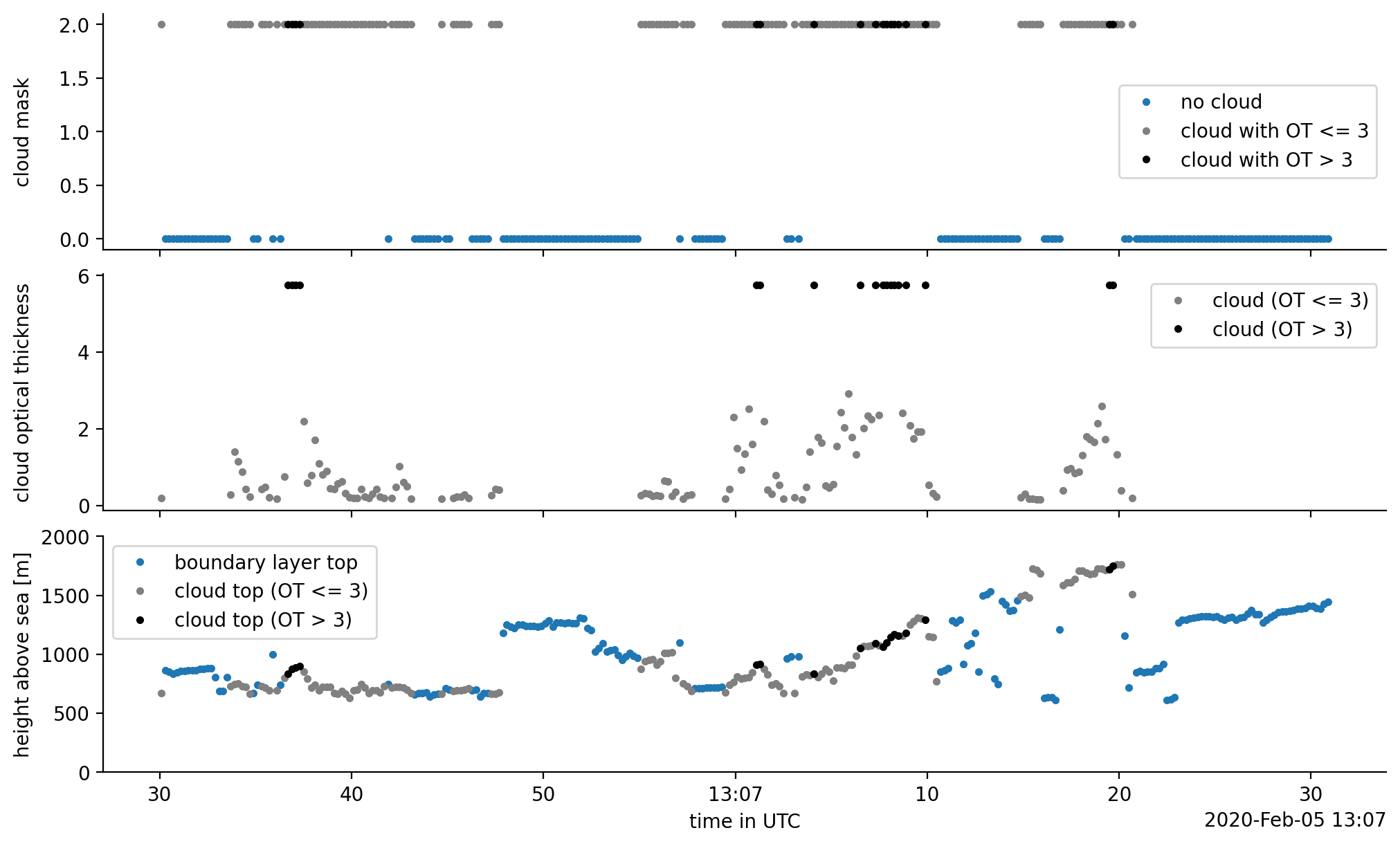
fig, axes = plt.subplots(3, 1, sharex=True)
ax1, ax2, ax3 = axes

cloud_free = ds_cloud_sel.cloud_mask[ds_cloud_sel.cloud_mask == cm_meanings["cloud_free"]]
cloud_free.plot(ax=ax1, x="time", ls="", marker=".", color="C0", label="no cloud")

thin_cloud = ds_cloud_sel.cloud_mask[ds_cloud_sel.cloud_ot<=3]
thin_cloud.plot(ax=ax1, x="time", ls="", marker=".", color="grey", label="cloud with OT <= 3")

thick_cloud = ds_cloud_sel.cloud_mask[ds_cloud_sel.cloud_ot>3]
thick_cloud.plot(ax=ax1, x="time", ls="", marker=".", color="k", label="cloud with OT > 3")

ax1.set_ylabel(f"{ds_cloud_sel.cloud_mask.long_name}")


ot_of_thin_cloud = ds_cloud_sel.cloud_ot[ds_cloud_sel.cloud_ot<=3]
ot_of_thin_cloud.plot(ax=ax2, x="time", ls="", marker=".", color="grey", label="cloud (OT <= 3)")

ot_of_thick_cloud = ds_cloud_sel.cloud_ot[ds_cloud_sel.cloud_ot>3]
ot_of_thick_cloud.plot(ax=ax2, x="time", ls="", marker=".", color="k", label="cloud (OT > 3)")

ax2.set_ylabel(f"{ds_cloud_sel.cloud_ot.long_name}")


pbl_top = ds_cloud_sel.pbl_top
pbl_top.plot(ax=ax3, x="time", ls="", marker=".", color="C0", label="boundary layer top")

thin_cloud_top = ds_cloud_sel.cloud_top[ds_cloud_sel.cloud_ot<=3]
thin_cloud_top.plot(ax=ax3, x="time", ls="", marker=".", color="grey", label="cloud top (OT <= 3)")

thick_cloud_top = ds_cloud_sel.cloud_top[ds_cloud_sel.cloud_ot>3]
thick_cloud_top.plot(ax=ax3, x="time", ls="", marker=".", color="k", label="cloud top (OT > 3)")

ax3.set_ylim(0, 2000)
ax3.set_ylabel("height above sea [m]")
ax3.set_xlabel('time in UTC')

for ax in axes:
    ax.label_outer()
    ax.legend()

fig.align_ylabels()
None

Cloud fraction

The cloud fraction can be estimated based on how often the instrument detected a cloud versus how often it measured anything. So, in order to compute the cloud fraction correctly, we must take care of missing values, in the original dataset. As Python has no commonly used way of carrying on a missing value through comparisions, we must keep track of it ourselves.

Note

In contrary, the R language for example knows about the special value NA which is carried along through compatisons, such that the result of the comparison NA == 3 continues to be NA.

In Python and in particular using xarray, missing data is expressed as np.nan, and due to floating point rules np.nan == 3 evaluates to False. As this False value is indistinguishable from a value which didn’t match out flag (3 in this case), averaging over the result would lead to a wrong cloud fraction result.

To keep track of the missing data, we’ll use DataArray.where on our boolean results to convert the results back to floating-point numbers (0 and 1) and fill missing values back in as np.nan. Later on, methods like .sum() and .mean() will automatically skip the np.nan values such that our results will be correct. To finally compute the cloud fraction, we need some form of binary cloud mask, which contains values of either 0 or one. To do so, we have two options, depending on whether we want to include 'probably_cloudy' or not. These two options are denoted by min_ (without probably cloudy) and max_ (with probably cloudy) prefixes.

cloudy_flags = xr.DataArray(
    [cm_meanings['probably_cloudy'], cm_meanings['most_likely_cloudy']],
    dims=("flags",))

min_cloud_binary_mask = (ds_cloud.cloud_mask == cm_meanings['most_likely_cloudy']).where(ds_cloud.cloud_mask.notnull())
max_cloud_binary_mask = (ds_cloud.cloud_mask == cloudy_flags).any("flags").where(ds_cloud.cloud_mask.notnull())
cloud_ot_gt3 = (ds_cloud.cloud_ot > 3).where(ds_cloud.cloud_ot.notnull())

print(f"Minimum cloud fraction on Feb 5: {min_cloud_binary_mask.mean().values * 100:.2f} %")
print(f"Total cloud fraction on Feb 5: {max_cloud_binary_mask.mean().values * 100:.2f} %")
print(f"Fraction of clouds with optical thickness greater than 3: {cloud_ot_gt3.mean().values * 100:.2f} %")

Minimum cloud fraction on Feb 5: 40.23 %
Total cloud fraction on Feb 5: 40.23 %

Fraction of clouds with optical thickness greater than 3: 28.25 %

As it turns out, in this section of the flight, the instrument is very certain about the cloudiness. Yet, this missing value story was a bit complicated, so let’s check if we would get something different if we would do it the naive way:

cf_wrong = (ds_cloud.cloud_mask == cloudy_flags).any("flags").mean().values
print(f"wrong cloud fraction: {cf_wrong * 100:.2f} %")

wrong cloud fraction: 39.93 %

Indeed, this is different… Good that we have thought about it.

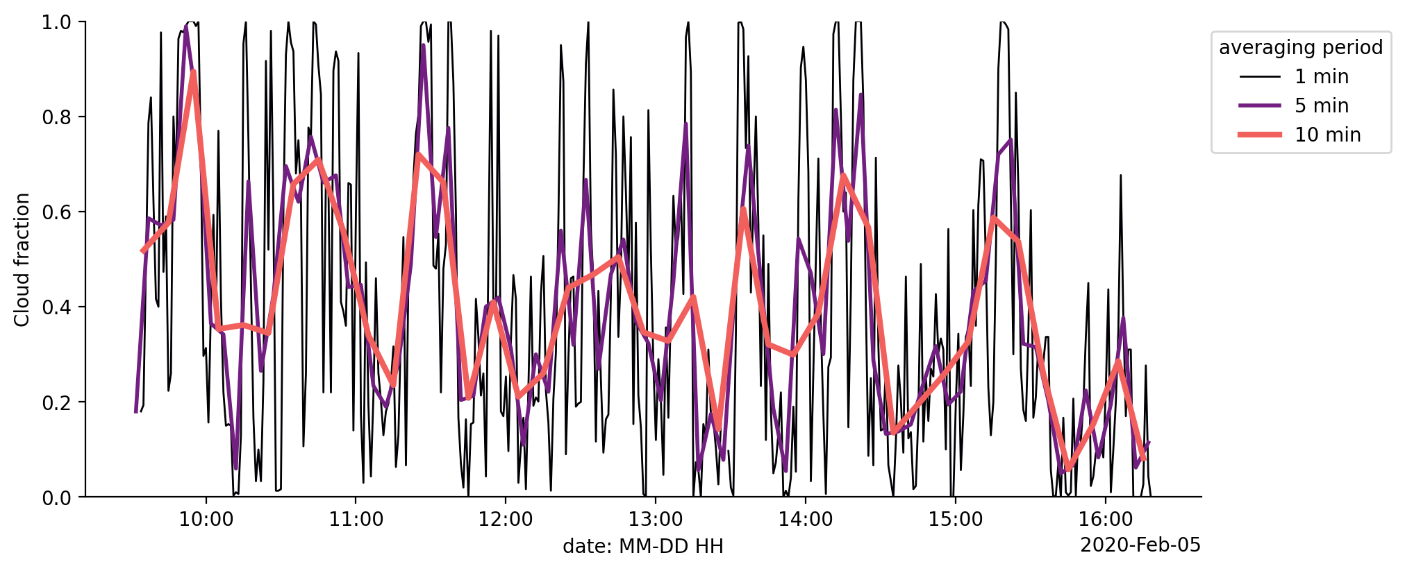
We can now use a time averaging window to derive a time dependent cloud fraction from the cloud_mask variable and see how it varies over the course of the flight.

with plt.style.context("mplstyle/wide"):
    fig, ax = plt.subplots()

    ax.set_prop_cycle(color=plt.get_cmap("magma")(np.linspace(0, 1, 4)))
    for ind, t in enumerate([1, 5, 10]):
        averaged_cloud_fraction = min_cloud_binary_mask.resample(time=f"{t}min", loffset=f"{t/2}min").mean()
        averaged_cloud_fraction.plot(lw=ind + 1, label=f"{t} min")

    ax.set_ylim(0, 1)
    ax.set_ylabel("Cloud fraction")
    ax.set_xlabel("date: MM-DD HH")
    ax.legend(title="averaging period", bbox_to_anchor=(1,1), loc="upper left")
    None

<string>:10: FutureWarning: Following pandas, the `loffset` parameter to resample is deprecated.  Switch to updating the resampled dataset time coordinate using time offset arithmetic.  For example:
    >>> offset = pd.tseries.frequencies.to_offset(freq) / 2
    >>> resampled_ds["time"] = resampled_ds.get_index("time") + offset

<string>:10: FutureWarning: Following pandas, the `loffset` parameter to resample is deprecated.  Switch to updating the resampled dataset time coordinate using time offset arithmetic.  For example:
    >>> offset = pd.tseries.frequencies.to_offset(freq) / 2
    >>> resampled_ds["time"] = resampled_ds.get_index("time") + offset
<string>:10: FutureWarning: Following pandas, the `loffset` parameter to resample is deprecated.  Switch to updating the resampled dataset time coordinate using time offset arithmetic.  For example:
    >>> offset = pd.tseries.frequencies.to_offset(freq) / 2
    >>> resampled_ds["time"] = resampled_ds.get_index("time") + offset