WSRA example: surface wave state#
During EUREC⁴A/ATOMIC the P-3 flew with a Wide Swath Radar Altimeter (WSRA), a digital beam-forming radar altimeter operating at 16 GHz in the Ku band. It generates 80 narrow beams spread over 30 deg to produce a topographic map of the sea surface waves and their backscattered power. These measurements allow for continuous reporting of directional ocean wave spectra and quantities derived from this including significant wave height, sea surface mean square slope, and the height, wavelength, and direction of propagation of primary and secondary wave fields. WSRA measurements are processed by the private company ProSensing, which designed and built the instrument.
The WSRA also produces rainfall rate estimates from path-integrated attenuation but we won’t look at those here.
The data are available through the EUREC⁴A intake catalog.
import xarray as xr
import numpy as np

import matplotlib.pyplot as plt
import pathlib
plt.style.use(pathlib.Path("./mplstyle/book"))
import colorcet as cc
%matplotlib inline

import eurec4a
cat = eurec4a.get_intake_catalog(use_ipfs="QmahMN2wgPauHYkkiTGoG2TpPBmj3p5FoYJAq9uE9iXT9N")
Mapping takes quite some setup. Maybe we’ll encapsulate this later but for now we repeat code in each notebook.
We’ll select an hour’s worth of observations from a single flight day. WSRA data are stored as “trajectories” - discrete times with associated positions and observations.
wsra_example = cat.P3.wsra["P3-0119"].to_dask().sel(trajectory=slice(0,293))
/home/runner/miniconda3/envs/how_to_eurec4a/lib/python3.13/site-packages/intake_xarray/base.py:21: FutureWarning: The return type of `Dataset.dims` will be changed to return a set of dimension names in future, in order to be more consistent with `DataArray.dims`. To access a mapping from dimension names to lengths, please use `Dataset.sizes`.
  'dims': dict(self._ds.dims),
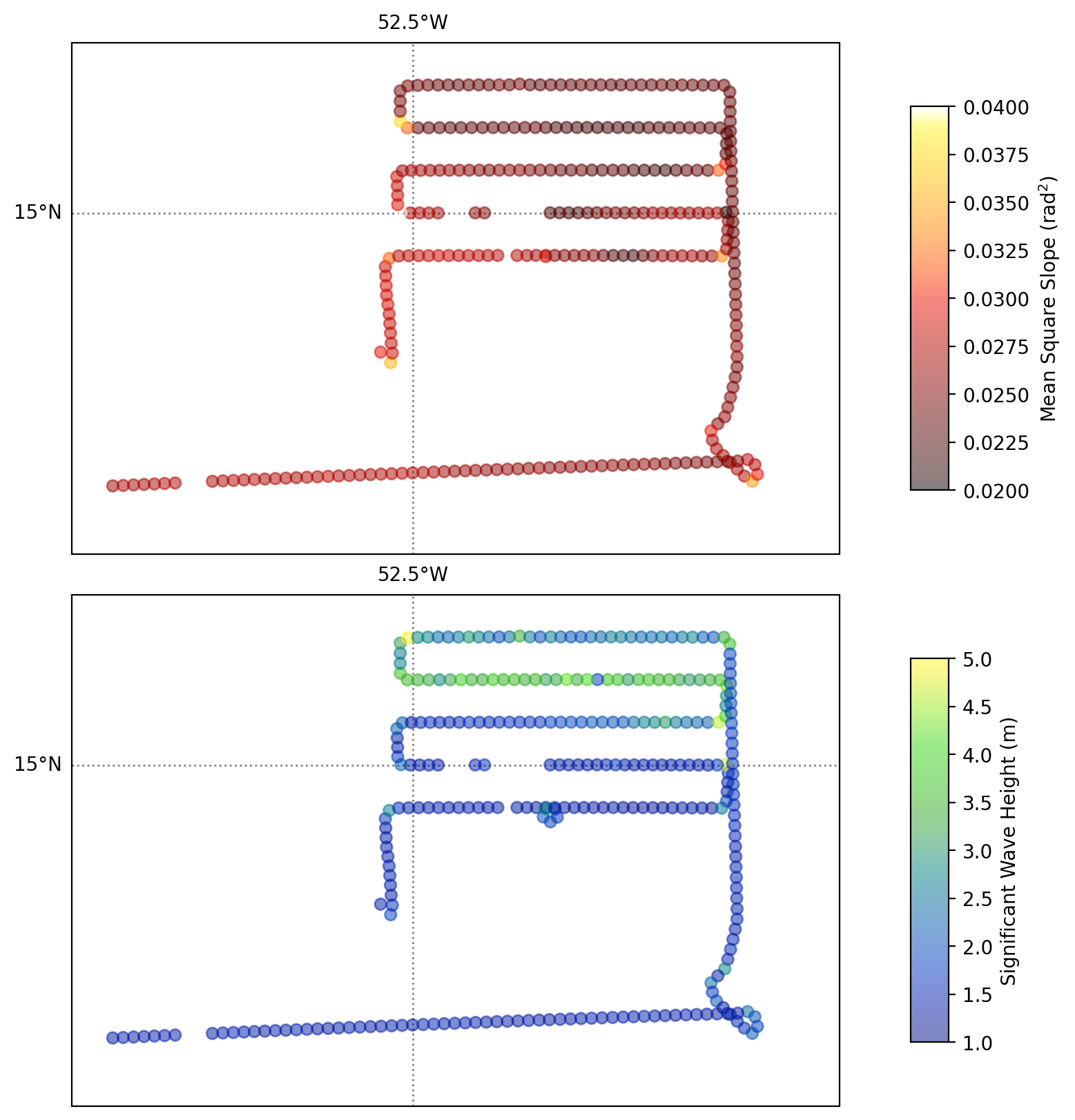
Now it’s interesting to see how the wave slope (top panel) and the wave height (bottom) vary spatially on a given day.
fig, (ax1, ax2) = plt.subplots(nrows=2, sharex = True, figsize = (12,8),
                               subplot_kw={'projection': ccrs.PlateCarree()})

#
# Mean square slope
#
ax_to_map(ax1, lon_e=-50, lon_w=-54.5, lat_s = 13, lat_n = 16)
add_gridlines(ax1)
pts = ax1.scatter(wsra_example.longitude,wsra_example.latitude,
           c=wsra_example.sea_surface_mean_square_slope_median,
           vmin = 0.02, vmax=0.04,
           cmap=cc.cm.fire,
           alpha=0.5,
           transform=ccrs.PlateCarree(),zorder=7)
fig.colorbar(pts, ax=ax1, shrink=0.75, aspect=10, label="Mean Square Slope (rad$^2$)")
#
# Significant wave height
#
ax_to_map(ax2, lon_e=-50, lon_w=-54.5, lat_s = 13, lat_n = 16)
add_gridlines(ax2)
pts = ax2.scatter(wsra_example.longitude,wsra_example.latitude,
           c=wsra_example.sea_surface_wave_significant_height,
           vmin = 1, vmax=5,
           cmap=cc.cm.bgy,
           alpha=0.5,
           transform=ccrs.PlateCarree(),zorder=7)
fig.colorbar(pts, ax=ax2, shrink=0.75, aspect=10, label="Significant Wave Height (m)");