interactive HALO tracks

This notebook shows how to plot the flight tracks of the HALO aircraft. First, we’ll have only a quick look and later on we do some more work in order to get the data onto an interactive map.

Preparations

First, we’ll import pylab and the EUREC4A data catalog.

import eurec4a
cat = eurec4a.get_intake_catalog(use_ipfs="QmahMN2wgPauHYkkiTGoG2TpPBmj3p5FoYJAq9uE9iXT9N")

Inspecting the dataset

ds = cat.HALO.BAHAMAS.PositionAttitude['HALO-0122'].to_dask()
ds

/usr/share/miniconda3/envs/how_to_eurec4a/lib/python3.12/site-packages/intake_xarray/base.py:21: FutureWarning: The return type of `Dataset.dims` will be changed to return a set of dimension names in future, in order to be more consistent with `DataArray.dims`. To access a mapping from dimension names to lengths, please use `Dataset.sizes`.
  'dims': dict(self._ds.dims),

<xarray.Dataset> Size: 15MB
Dimensions:     (time: 331760)
Coordinates:
    alt         (time) float32 1MB dask.array<chunksize=(82940,), meta=np.ndarray>
    lat         (time) float64 3MB dask.array<chunksize=(41470,), meta=np.ndarray>
    lon         (time) float64 3MB dask.array<chunksize=(41470,), meta=np.ndarray>
  * time        (time) datetime64[ns] 3MB 2020-01-22T14:57:36 ... 2020-01-23T...
Data variables:
    heading     (time) float32 1MB dask.array<chunksize=(82940,), meta=np.ndarray>
    pitch       (time) float32 1MB dask.array<chunksize=(82940,), meta=np.ndarray>
    roll        (time) float32 1MB dask.array<chunksize=(82940,), meta=np.ndarray>
    tas         (time) float32 1MB dask.array<chunksize=(82940,), meta=np.ndarray>
    trajectory  <U4 16B ...
Attributes: (12/13)
    Conventions:        CF-1.7
    date_last_revised:  2020-4-16
    description:        10Hz subset based on DLR BAHAMAS data, processed by A...
    featureType:        trajectory
    file_created:       File created by M. Klingebiel (email: marcus.klingebi...
    flight_id:          HALO-0122
    ...                 ...
    instrument:         BAHAMAS
    mission:            EUREC4A
    platform:           HALO
    source_file:        HALO-DB_dataset7374_release1_EUREC4A_HALO_BAHAMAS10Hz...
    title:              EUREC4A position and attitude data
    version:            1.1

xarray.Dataset

• Dimensions:
  • time: 331760
• Coordinates: (4)
  • alt
    (time)
    float32
    dask.array<chunksize=(82940,), meta=np.ndarray>

    axis :

    Z

    long_name :

    WGS84 Datum/Elliptical Height

    positive :

    up

    standard_name :

    height_above_reference_ellipsoid

    units :

    m

    Array Chunk Bytes 1.27 MiB 323.98 kiB Shape (331760,) (82940,) Dask graph 4 chunks in 2 graph layers Data type float32 numpy.ndarray

  • lat
    (time)
    float64
    dask.array<chunksize=(41470,), meta=np.ndarray>

    axis :

    Y

    long_name :

    WGS84 Datum/Latitude

    standard_name :

    latitude

    units :

    degrees_north

    Array Chunk Bytes 2.53 MiB 323.98 kiB Shape (331760,) (41470,) Dask graph 8 chunks in 2 graph layers Data type float64 numpy.ndarray

  • lon
    (time)
    float64
    dask.array<chunksize=(41470,), meta=np.ndarray>

    axis :

    X

    long_name :

    WGS84 Datum/Longitude

    standard_name :

    longitude

    units :

    degrees_east

    Array Chunk Bytes 2.53 MiB 323.98 kiB Shape (331760,) (41470,) Dask graph 8 chunks in 2 graph layers Data type float64 numpy.ndarray

  • time
    (time)
    datetime64[ns]
    2020-01-22T14:57:36 ... 2020-01-...

    axis :

    T

    long_name :

    Time in seconds since 2020-1-1

    standard_name :

    time

    array(['2020-01-22T14:57:36.000000000', '2020-01-22T14:57:36.099999904',
           '2020-01-22T14:57:36.200000047', ..., '2020-01-23T00:10:31.700000047',
           '2020-01-23T00:10:31.799999952', '2020-01-23T00:10:31.900000095'],
          dtype='datetime64[ns]')

• Data variables: (5)
  • heading
    (time)
    float32
    dask.array<chunksize=(82940,), meta=np.ndarray>

    long_name :

    true heading

    standard_name :

    platform_yaw_fore_starboard

    units :

    degrees

    Array Chunk Bytes 1.27 MiB 323.98 kiB Shape (331760,) (82940,) Dask graph 4 chunks in 2 graph layers Data type float32 numpy.ndarray

  • pitch
    (time)
    float32
    dask.array<chunksize=(82940,), meta=np.ndarray>

    long_name :

    pitch angle

    standard_name :

    platform_pitch_fore_up

    units :

    degrees

    Array Chunk Bytes 1.27 MiB 323.98 kiB Shape (331760,) (82940,) Dask graph 4 chunks in 2 graph layers Data type float32 numpy.ndarray

  • roll
    (time)
    float32
    dask.array<chunksize=(82940,), meta=np.ndarray>

    long_name :

    roll angle

    standard_name :

    platform_roll_starboard_down

    units :

    degrees

    Array Chunk Bytes 1.27 MiB 323.98 kiB Shape (331760,) (82940,) Dask graph 4 chunks in 2 graph layers Data type float32 numpy.ndarray

  • tas
    (time)
    float32
    dask.array<chunksize=(82940,), meta=np.ndarray>

    long_name :

    Calculated True Airspeed

    standard_name :

    platform_speed_wrt_air

    units :

    m/s

    Array Chunk Bytes 1.27 MiB 323.98 kiB Shape (331760,) (82940,) Dask graph 4 chunks in 2 graph layers Data type float32 numpy.ndarray

  • trajectory
    ()
    <U4
    ...

    cf_role :

    trajectory_id

    description :

    platform id, unique string describing the trajectory

    long_name :

    trajectory identifier

    [1 values with dtype=<U4]

• Indexes: (1)
  • time
    PandasIndex

    PandasIndex(DatetimeIndex([          '2020-01-22 14:57:36',
                   '2020-01-22 14:57:36.099999904',
                   '2020-01-22 14:57:36.200000047',
                   '2020-01-22 14:57:36.299999952',
                   '2020-01-22 14:57:36.400000095',
                      '2020-01-22 14:57:36.500000',
                   '2020-01-22 14:57:36.599999904',
                   '2020-01-22 14:57:36.700000047',
                   '2020-01-22 14:57:36.799999952',
                   '2020-01-22 14:57:36.900000095',
                   ...
                             '2020-01-23 00:10:31',
                   '2020-01-23 00:10:31.099999904',
                   '2020-01-23 00:10:31.200000047',
                   '2020-01-23 00:10:31.299999952',
                   '2020-01-23 00:10:31.400000095',
                      '2020-01-23 00:10:31.500000',
                   '2020-01-23 00:10:31.599999904',
                   '2020-01-23 00:10:31.700000047',
                   '2020-01-23 00:10:31.799999952',
                   '2020-01-23 00:10:31.900000095'],
                  dtype='datetime64[ns]', name='time', length=331760, freq=None))

• Attributes: (13)

  Conventions :

  CF-1.7

  date_last_revised :

  2020-4-16

  description :

  10Hz subset based on DLR BAHAMAS data, processed by A. Giez, V. Dreiling, M. Zoeger, Ch. Mallaun; email: andreas.giez@dlr.de

  featureType :

  trajectory

  file_created :

  File created by M. Klingebiel (email: marcus.klingebiel@uni-leipzig.de) on March 09, 2021

  flight_id :

  HALO-0122

  history :

  acquired by HALO BAHAMAS, processed and quality checked by DLR FX, subsetted and reformatted by Marcus Klingebiel, time had an offset by one hour in v1.0 which is corrected in v1.1

  instrument :

  BAHAMAS

  mission :

  EUREC4A

  platform :

  HALO

  source_file :

  HALO-DB_dataset7374_release1_EUREC4A_HALO_BAHAMAS10Hz_20200122a.nc

  title :

  EUREC4A position and attitude data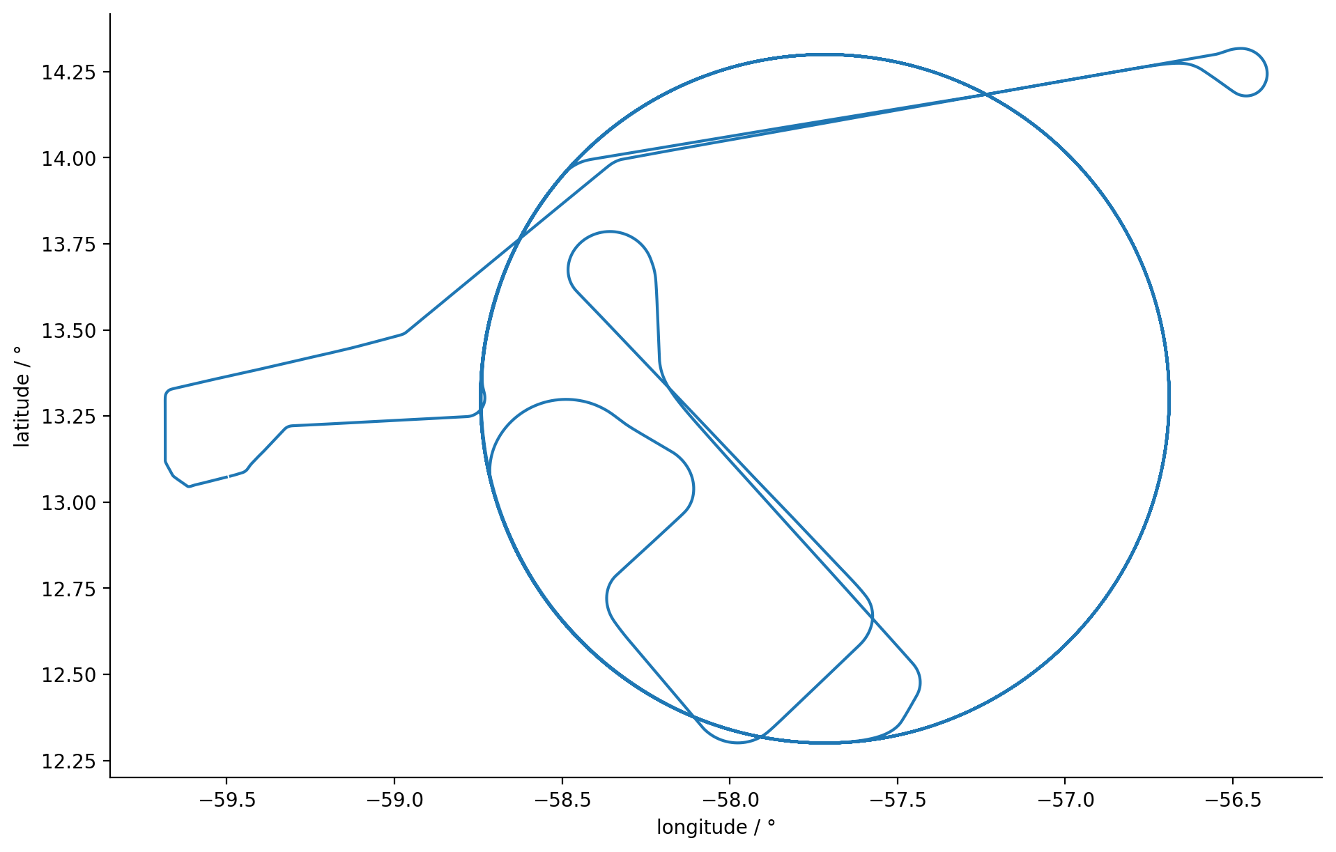

  version :

  1.1

Just to have a better visual impression, we can create a quick overview plot of the data:

%matplotlib inline
import numpy as np
import matplotlib.pyplot as plt
import pathlib
plt.style.use(pathlib.Path("./mplstyle/book"))

plt.plot(ds.lon, ds.lat)
center_lat = float(ds.lat.mean())
plt.gca().set_aspect(1./np.cos(np.deg2rad(center_lat)))
plt.xlabel("longitude / °")
plt.ylabel("latitude / °")
plt.show()

Reducing the size of the dataset

Later on, we want to plot all flights on an interactive map. Currently the dataset is rather large as the aircraft location has been recorded continuously at a high data rate. While this is good for quantitative analysis, this leads to poor interactive performance. So before going further, it is a good idea to reduce the amount of data while keeping the visual impression.

A possible idea to reduce the amount of required data is that plotting a line already does linear interpolation between two coordinate points. So if we would remove those points which are close to the linear interpolation between its neighboring points, the visual impression will stay almost the same. This idea has already been stated by Ramer Douglas and Peucker and is illustrated at Wikipedia. While the algorithm is not hard to write, it is difficult to do it efficiently in python. Thus, I’ve skipped it and use the simplification library in stead.

Note

Many algorithms for shape processing are contained in the beautiful shapely library. In general, I’d recommend using that library, but it requies the GEOS library which is a bit tricky to install.

from simplification.cutil import simplify_coords_idx
def simplify_dataset(ds, tolerance):
    indices_to_take = simplify_coords_idx(np.stack([ds.lat.values, ds.lon.values], axis=1), tolerance)
    return ds.isel(time=indices_to_take)

We can now use that algorithm to generate a simplified version of the dataset with a tolerance of \(10^{-5}\) degrees, which otherwise looks the same to the previous version.

dssimplified = simplify_dataset(ds, 1e-5)
dssimplified

<xarray.Dataset> Size: 362kB
Dimensions:     (time: 8225)
Coordinates:
    alt         (time) float32 33kB dask.array<chunksize=(2451,), meta=np.ndarray>
    lat         (time) float64 66kB dask.array<chunksize=(1264,), meta=np.ndarray>
    lon         (time) float64 66kB dask.array<chunksize=(1264,), meta=np.ndarray>
  * time        (time) datetime64[ns] 66kB 2020-01-22T14:57:36 ... 2020-01-23...
Data variables:
    heading     (time) float32 33kB dask.array<chunksize=(2451,), meta=np.ndarray>
    pitch       (time) float32 33kB dask.array<chunksize=(2451,), meta=np.ndarray>
    roll        (time) float32 33kB dask.array<chunksize=(2451,), meta=np.ndarray>
    tas         (time) float32 33kB dask.array<chunksize=(2451,), meta=np.ndarray>
    trajectory  <U4 16B ...
Attributes: (12/13)
    Conventions:        CF-1.7
    date_last_revised:  2020-4-16
    description:        10Hz subset based on DLR BAHAMAS data, processed by A...
    featureType:        trajectory
    file_created:       File created by M. Klingebiel (email: marcus.klingebi...
    flight_id:          HALO-0122
    ...                 ...
    instrument:         BAHAMAS
    mission:            EUREC4A
    platform:           HALO
    source_file:        HALO-DB_dataset7374_release1_EUREC4A_HALO_BAHAMAS10Hz...
    title:              EUREC4A position and attitude data
    version:            1.1

xarray.Dataset

• Dimensions:
  • time: 8225
• Coordinates: (4)
  • alt
    (time)
    float32
    dask.array<chunksize=(2451,), meta=np.ndarray>

    axis :

    Z

    long_name :

    WGS84 Datum/Elliptical Height

    positive :

    up

    standard_name :

    height_above_reference_ellipsoid

    units :

    m

    Array Chunk Bytes 32.13 kiB 9.57 kiB Shape (8225,) (2451,) Dask graph 4 chunks in 3 graph layers Data type float32 numpy.ndarray

  • lat
    (time)
    float64
    dask.array<chunksize=(1264,), meta=np.ndarray>

    axis :

    Y

    long_name :

    WGS84 Datum/Latitude

    standard_name :

    latitude

    units :

    degrees_north

    Array Chunk Bytes 64.26 kiB 10.63 kiB Shape (8225,) (1361,) Dask graph 8 chunks in 3 graph layers Data type float64 numpy.ndarray

  • lon
    (time)
    float64
    dask.array<chunksize=(1264,), meta=np.ndarray>

    axis :

    X

    long_name :

    WGS84 Datum/Longitude

    standard_name :

    longitude

    units :

    degrees_east

    Array Chunk Bytes 64.26 kiB 10.63 kiB Shape (8225,) (1361,) Dask graph 8 chunks in 3 graph layers Data type float64 numpy.ndarray

  • time
    (time)
    datetime64[ns]
    2020-01-22T14:57:36 ... 2020-01-...

    axis :

    T

    long_name :

    Time in seconds since 2020-1-1

    standard_name :

    time

    array(['2020-01-22T14:57:36.000000000', '2020-01-22T14:57:44.000000000',
           '2020-01-22T14:57:49.599999904', ..., '2020-01-23T00:10:01.700000047',
           '2020-01-23T00:10:16.700000047', '2020-01-23T00:10:31.900000095'],
          dtype='datetime64[ns]')

• Data variables: (5)
  • heading
    (time)
    float32
    dask.array<chunksize=(2451,), meta=np.ndarray>

    long_name :

    true heading

    standard_name :

    platform_yaw_fore_starboard

    units :

    degrees

    Array Chunk Bytes 32.13 kiB 9.57 kiB Shape (8225,) (2451,) Dask graph 4 chunks in 3 graph layers Data type float32 numpy.ndarray

  • pitch
    (time)
    float32
    dask.array<chunksize=(2451,), meta=np.ndarray>

    long_name :

    pitch angle

    standard_name :

    platform_pitch_fore_up

    units :

    degrees

    Array Chunk Bytes 32.13 kiB 9.57 kiB Shape (8225,) (2451,) Dask graph 4 chunks in 3 graph layers Data type float32 numpy.ndarray

  • roll
    (time)
    float32
    dask.array<chunksize=(2451,), meta=np.ndarray>

    long_name :

    roll angle

    standard_name :

    platform_roll_starboard_down

    units :

    degrees

    Array Chunk Bytes 32.13 kiB 9.57 kiB Shape (8225,) (2451,) Dask graph 4 chunks in 3 graph layers Data type float32 numpy.ndarray

  • tas
    (time)
    float32
    dask.array<chunksize=(2451,), meta=np.ndarray>

    long_name :

    Calculated True Airspeed

    standard_name :

    platform_speed_wrt_air

    units :

    m/s

    Array Chunk Bytes 32.13 kiB 9.57 kiB Shape (8225,) (2451,) Dask graph 4 chunks in 3 graph layers Data type float32 numpy.ndarray

  • trajectory
    ()
    <U4
    ...

    cf_role :

    trajectory_id

    description :

    platform id, unique string describing the trajectory

    long_name :

    trajectory identifier

    [1 values with dtype=<U4]

• Indexes: (1)
  • time
    PandasIndex

    PandasIndex(DatetimeIndex([          '2020-01-22 14:57:36',
                             '2020-01-22 14:57:44',
                   '2020-01-22 14:57:49.599999904',
                   '2020-01-22 14:57:54.400000095',
                   '2020-01-22 14:58:08.299999952',
                      '2020-01-22 14:58:15.500000',
                             '2020-01-22 14:58:17',
                   '2020-01-22 14:58:18.200000047',
                             '2020-01-22 14:58:20',
                   '2020-01-22 14:58:21.700000047',
                   ...
                   '2020-01-23 00:08:10.200000047',
                   '2020-01-23 00:08:14.799999952',
                   '2020-01-23 00:08:30.799999952',
                   '2020-01-23 00:08:42.900000095',
                   '2020-01-23 00:08:55.400000095',
                      '2020-01-23 00:09:09.500000',
                   '2020-01-23 00:09:42.599999904',
                   '2020-01-23 00:10:01.700000047',
                   '2020-01-23 00:10:16.700000047',
                   '2020-01-23 00:10:31.900000095'],
                  dtype='datetime64[ns]', name='time', length=8225, freq=None))

• Attributes: (13)

  Conventions :

  CF-1.7

  date_last_revised :

  2020-4-16

  description :

  10Hz subset based on DLR BAHAMAS data, processed by A. Giez, V. Dreiling, M. Zoeger, Ch. Mallaun; email: andreas.giez@dlr.de

  featureType :

  trajectory

  file_created :

  File created by M. Klingebiel (email: marcus.klingebiel@uni-leipzig.de) on March 09, 2021

  flight_id :

  HALO-0122

  history :

  acquired by HALO BAHAMAS, processed and quality checked by DLR FX, subsetted and reformatted by Marcus Klingebiel, time had an offset by one hour in v1.0 which is corrected in v1.1

  instrument :

  BAHAMAS

  mission :

  EUREC4A

  platform :

  HALO

  source_file :

  HALO-DB_dataset7374_release1_EUREC4A_HALO_BAHAMAS10Hz_20200122a.nc

  title :

  EUREC4A position and attitude data

  version :

  1.1

We can now compare those two tracks side by side while keeping a look at the number of data points required.

fig, (ax1, ax2) = plt.subplots(1, 2)
ax1.plot(ds.lon, ds.lat)
ax1.set_title(f"{len(ds.time)} data points")
ax2.plot(dssimplified.lon, dssimplified.lat)
ax2.set_title(f"{len(dssimplified.time)} data points")

for ax in (ax1, ax2):
    ax.set_aspect(1./np.cos(np.deg2rad(center_lat)))
    ax.set_xlabel("longitude / °")
    ax.set_ylabel("latitude / °")
    ax.label_outer()


plt.show()

ratio = len(dssimplified.time) / len(ds.time)
print(f"compression ratio: {ratio*100:.2f} %")

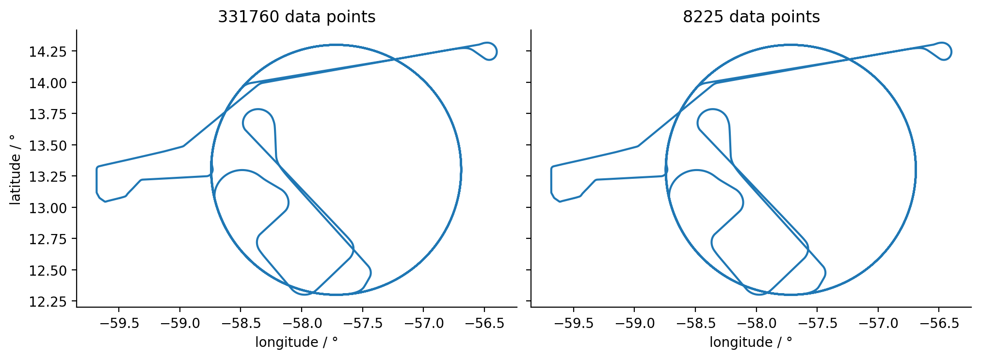
compression ratio: 2.48 %

The dataset size has been substantially reduced while the visual impression stayed the same.

First interactive map

In order to show the map a little bit more interactively, we use the ipyleaflet library which creates a bridge between ipython and the Leaflet JavaScript library.

import ipyleaflet

As we will need to convert many tracks to ipyleaflet layers later on, the easiest is to create a little function for that purpose right away:

def track2layer(track, color="green", name=""):
    return ipyleaflet.Polyline(
        locations=np.stack([track.lat.values, track.lon.values], axis=1).tolist(), 
        color=color,
        fill=False,
        weight=2,
        name=name
    )

With the help of that little function, creating a map is now like a breeze:

testmap = ipyleaflet.Map(center=(13.3, -57), zoom=7)
testmap.add_layer(track2layer(dssimplified))
display(testmap)

All in one

Let’s see if we can add all the flights and provide a layer switcher so that we can have a look at all flights individually. We’ll start by loading and simplifying all out track data into a local dictionary. Requesting the datasets from the server is IO bound and thus can simply be accellerated using a ThreadPool:

def get_dataset(flight_id):
    ds = cat.HALO.BAHAMAS.PositionAttitude[flight_id].to_dask()
    return ds[['lat','lon']].load()

full_tracks = {k: get_dataset(k) for k in cat.HALO.BAHAMAS.PositionAttitude}

/usr/share/miniconda3/envs/how_to_eurec4a/lib/python3.12/site-packages/intake_xarray/base.py:21: FutureWarning: The return type of `Dataset.dims` will be changed to return a set of dimension names in future, in order to be more consistent with `DataArray.dims`. To access a mapping from dimension names to lengths, please use `Dataset.sizes`.
  'dims': dict(self._ds.dims),

/usr/share/miniconda3/envs/how_to_eurec4a/lib/python3.12/site-packages/intake_xarray/base.py:21: FutureWarning: The return type of `Dataset.dims` will be changed to return a set of dimension names in future, in order to be more consistent with `DataArray.dims`. To access a mapping from dimension names to lengths, please use `Dataset.sizes`.
  'dims': dict(self._ds.dims),

/usr/share/miniconda3/envs/how_to_eurec4a/lib/python3.12/site-packages/intake_xarray/base.py:21: FutureWarning: The return type of `Dataset.dims` will be changed to return a set of dimension names in future, in order to be more consistent with `DataArray.dims`. To access a mapping from dimension names to lengths, please use `Dataset.sizes`.
  'dims': dict(self._ds.dims),

/usr/share/miniconda3/envs/how_to_eurec4a/lib/python3.12/site-packages/intake_xarray/base.py:21: FutureWarning: The return type of `Dataset.dims` will be changed to return a set of dimension names in future, in order to be more consistent with `DataArray.dims`. To access a mapping from dimension names to lengths, please use `Dataset.sizes`.
  'dims': dict(self._ds.dims),

/usr/share/miniconda3/envs/how_to_eurec4a/lib/python3.12/site-packages/intake_xarray/base.py:21: FutureWarning: The return type of `Dataset.dims` will be changed to return a set of dimension names in future, in order to be more consistent with `DataArray.dims`. To access a mapping from dimension names to lengths, please use `Dataset.sizes`.
  'dims': dict(self._ds.dims),

/usr/share/miniconda3/envs/how_to_eurec4a/lib/python3.12/site-packages/intake_xarray/base.py:21: FutureWarning: The return type of `Dataset.dims` will be changed to return a set of dimension names in future, in order to be more consistent with `DataArray.dims`. To access a mapping from dimension names to lengths, please use `Dataset.sizes`.
  'dims': dict(self._ds.dims),

/usr/share/miniconda3/envs/how_to_eurec4a/lib/python3.12/site-packages/intake_xarray/base.py:21: FutureWarning: The return type of `Dataset.dims` will be changed to return a set of dimension names in future, in order to be more consistent with `DataArray.dims`. To access a mapping from dimension names to lengths, please use `Dataset.sizes`.
  'dims': dict(self._ds.dims),

/usr/share/miniconda3/envs/how_to_eurec4a/lib/python3.12/site-packages/intake_xarray/base.py:21: FutureWarning: The return type of `Dataset.dims` will be changed to return a set of dimension names in future, in order to be more consistent with `DataArray.dims`. To access a mapping from dimension names to lengths, please use `Dataset.sizes`.
  'dims': dict(self._ds.dims),

/usr/share/miniconda3/envs/how_to_eurec4a/lib/python3.12/site-packages/intake_xarray/base.py:21: FutureWarning: The return type of `Dataset.dims` will be changed to return a set of dimension names in future, in order to be more consistent with `DataArray.dims`. To access a mapping from dimension names to lengths, please use `Dataset.sizes`.
  'dims': dict(self._ds.dims),

/usr/share/miniconda3/envs/how_to_eurec4a/lib/python3.12/site-packages/intake_xarray/base.py:21: FutureWarning: The return type of `Dataset.dims` will be changed to return a set of dimension names in future, in order to be more consistent with `DataArray.dims`. To access a mapping from dimension names to lengths, please use `Dataset.sizes`.
  'dims': dict(self._ds.dims),

/usr/share/miniconda3/envs/how_to_eurec4a/lib/python3.12/site-packages/intake_xarray/base.py:21: FutureWarning: The return type of `Dataset.dims` will be changed to return a set of dimension names in future, in order to be more consistent with `DataArray.dims`. To access a mapping from dimension names to lengths, please use `Dataset.sizes`.
  'dims': dict(self._ds.dims),

/usr/share/miniconda3/envs/how_to_eurec4a/lib/python3.12/site-packages/intake_xarray/base.py:21: FutureWarning: The return type of `Dataset.dims` will be changed to return a set of dimension names in future, in order to be more consistent with `DataArray.dims`. To access a mapping from dimension names to lengths, please use `Dataset.sizes`.
  'dims': dict(self._ds.dims),

/usr/share/miniconda3/envs/how_to_eurec4a/lib/python3.12/site-packages/intake_xarray/base.py:21: FutureWarning: The return type of `Dataset.dims` will be changed to return a set of dimension names in future, in order to be more consistent with `DataArray.dims`. To access a mapping from dimension names to lengths, please use `Dataset.sizes`.
  'dims': dict(self._ds.dims),

/usr/share/miniconda3/envs/how_to_eurec4a/lib/python3.12/site-packages/intake_xarray/base.py:21: FutureWarning: The return type of `Dataset.dims` will be changed to return a set of dimension names in future, in order to be more consistent with `DataArray.dims`. To access a mapping from dimension names to lengths, please use `Dataset.sizes`.
  'dims': dict(self._ds.dims),

/usr/share/miniconda3/envs/how_to_eurec4a/lib/python3.12/site-packages/intake_xarray/base.py:21: FutureWarning: The return type of `Dataset.dims` will be changed to return a set of dimension names in future, in order to be more consistent with `DataArray.dims`. To access a mapping from dimension names to lengths, please use `Dataset.sizes`.
  'dims': dict(self._ds.dims),

/usr/share/miniconda3/envs/how_to_eurec4a/lib/python3.12/site-packages/intake_xarray/base.py:21: FutureWarning: The return type of `Dataset.dims` will be changed to return a set of dimension names in future, in order to be more consistent with `DataArray.dims`. To access a mapping from dimension names to lengths, please use `Dataset.sizes`.
  'dims': dict(self._ds.dims),

We still have to simplify the dataset, which is done here:

tracks = {flight_id: simplify_dataset(ds, 1e-5)
          for flight_id, ds in full_tracks.items()}

Let’s also quickly grab some colors from a matplotlib colorbar, such that we can show all tracks in individual colors:

import matplotlib
colors = [matplotlib.colors.to_hex(c)
          for c in plt.cm.inferno(np.linspace(0, 1, len(tracks)))]

We can now start with a new empty map. Let’s also have a different basemap.

m = ipyleaflet.Map(
    basemap=ipyleaflet.basemaps.Esri.NatGeoWorldMap,
    center=(13.3, -57), zoom=7
)

We’ll add all the tracks as individual layers to the map

for (flight_id, track), color in zip(tracks.items(), colors):
    m.add_layer(track2layer(track, color, flight_id))

and add a scale, a legend, layer controls and a full screen button to the map and show it. If you want to zoom in, you can for example shift-click and drag a rectangle over the area you want to zoom in more closely.

m.add_control(ipyleaflet.ScaleControl(position='bottomleft'))
m.add_control(ipyleaflet.LegendControl(dict(zip(tracks, colors)),
                                       name="Flights",
                                       position="bottomright"))
m.add_control(ipyleaflet.LayersControl(position='topright'))
m.add_control(ipyleaflet.FullScreenControl())
display(m)