Cloud Botany with DALES#
Setup#
Cloud Botany is a library of idealised large-eddy simulations forced by and initialised with combinations of simplified vertical profiles. Each profile is parameterised by variables which aim to make the ensemble span a range of conditions corresponding to the variability observed over the EUREC4A region during the boreal winter of 2019/2020. The following table lists these varied parameters and their ranges:
variable |
min |
max |
unit |
description |
|---|---|---|---|---|
|
297.5 |
299.5 |
K |
sea surface potential temperature |
|
-5 |
-15 |
m/s |
surface wind |
|
0.0135 |
0.015 |
kg/kg |
mixed-layer total specific humidity |
|
1200 |
2500 |
m |
humidity scale height |
|
4.5 |
5.5 |
K/km |
lapse rate of |
|
-0.35 |
0.18 |
cm/s |
Amplitude of subsidence first mode |
|
-0.0044 |
0.0044 |
1/s |
Wind shear[1] |
Availability of simulation output#
Cloud Botany contains simulations at a variety of grid resolutions and domain sizes, and each set of simulations comes with its own output. Most of this output is hosted and made available through DKRZ’s Swiftbrowser, and can be accessed through the eurec4a-intake catalog.
import eurec4a
cat = eurec4a.get_intake_catalog()
botany_cat = cat.simulations.DALES.botany
An overview over what is currently available through this structure is listed under Simulations, and is repeated below for convenience:
dx100m
   nx1536
      profiles
      timeseries
      2D
      3D
      cross_xy
      radiation
      parameters
   nx96
      profiles
      timeseries
      2D
      3D
      cross_xy
      radiation
      parameters
Output description#
Parameters#
A combination of grid resolution and domain size, e.g. botany_cat.dx100.nx1536, contains its own ensemble of cases. So far, two complete ensembles have been simulated, both at the grid spacing dx100: nx96 (9.6 km domain size) and nx1536 (153.6 km domain size). Both ensembles can be accessed through the eurec4a-intake catalog. Other grid configurations might be added at a later stage.
To inspect and use the nx1536 ensemble, start by loading its parameters:
import pandas as pd
varied_parameters = ['member','thls', 'u0', 'qt0', 'qt_lambda', 'thl_Gamma', 'wpamp', 'dudz', 'location']
parameters = cat.simulations.DALES.botany.dx100m.nx1536.parameters.read()
df_parameters = pd.DataFrame.from_records(parameters)[varied_parameters]
df_parameters
| member | thls | u0 | qt0 | qt_lambda | thl_Gamma | wpamp | dudz | location | |
|---|---|---|---|---|---|---|---|---|---|
| 0 | 1 | 298.5 | -10.0 | 0.01425 | 1850.0 | 5.0 | -0.00085 | 0.0022 | center |
| 1 | 2 | 297.5 | -15.0 | 0.01350 | 1200.0 | 4.5 | -0.00350 | 0.0022 | corner |
| 2 | 3 | 297.5 | -15.0 | 0.01350 | 1200.0 | 4.5 | 0.00180 | 0.0022 | corner |
| 3 | 4 | 297.5 | -15.0 | 0.01350 | 1200.0 | 5.5 | -0.00350 | 0.0022 | corner |
| 4 | 5 | 297.5 | -15.0 | 0.01350 | 1200.0 | 5.5 | 0.00180 | 0.0022 | corner |
| ... | ... | ... | ... | ... | ... | ... | ... | ... | ... |
| 98 | 99 | 298.5 | -10.0 | 0.01425 | 2200.0 | 5.0 | -0.00085 | 0.0022 | sweep qt_lambda |
| 99 | 100 | 298.5 | -10.0 | 0.01425 | 2500.0 | 5.0 | -0.00085 | 0.0022 | sweep qt_lambda |
| 100 | 101 | 298.5 | -10.0 | 0.01425 | 3000.0 | 5.0 | -0.00085 | 0.0022 | sweep qt_lambda |
| 101 | 102 | 298.5 | -10.0 | 0.01350 | 1850.0 | 5.0 | -0.00085 | 0.0022 | sweep qt0 |
| 102 | 103 | 298.5 | -10.0 | 0.01500 | 1850.0 | 5.0 | -0.00085 | 0.0022 | sweep qt0 |
103 rows × 9 columns
parameters contains the value of the variables in Table 1, as they vary for each member of the ensemble. The ensemble may be thought of a hypercube in the six-dimensional space spanned by [thls, u0, qt0, qt_lambda, thl_Gamma, wpamp]. The location column indicates where any member fits in this space:
The hypercube
centerrepresents the middle of the range between the minimum and maximum value of each variableThe hypercube
corners are constructed by evaluating all parameter combinations at their minimum and maximum (resulting in the next \(2^6 = 64\) simulations).Simulations belonging to a
sweephave a single variable vary between its minimum and maximum, while keeping all other variables constant at theircentervalue.
Simulation output#
The actual output from the simulations is stored in the other data sets in the tree listing above. Such data sets can be loaded according to the following example:
import xarray as xr

ds_profiles = botany_cat.dx100m.nx1536['profiles'].to_dask()
ds_profiles
/home/runner/miniconda3/envs/how_to_eurec4a/lib/python3.13/site-packages/intake_xarray/base.py:21: FutureWarning: The return type of `Dataset.dims` will be changed to return a set of dimension names in future, in order to be more consistent with `DataArray.dims`. To access a mapping from dimension names to lengths, please use `Dataset.sizes`.
  'dims': dict(self._ds.dims),
<xarray.Dataset> Size: 5GB
Dimensions:    (member: 103, time: 720, zt: 175, zm: 175)
Coordinates:
  * member     (member) int32 412B 1 2 3 4 5 6 7 8 ... 97 98 99 100 101 102 103
  * time       (time) datetime64[ns] 6kB 2020-02-01T00:05:00 ... 2020-02-03T1...
  * zm         (zm) float32 700B 0.0 15.0 30.0 ... 6.772e+03 6.854e+03 6.938e+03
  * zt         (zt) float32 700B 7.5 22.5 37.65 ... 6.813e+03 6.896e+03 6.98e+03
Data variables: (12/102)
    cfrac      (member, time, zt) float32 52MB dask.array<chunksize=(32, 256, 175), meta=np.ndarray>
    cs         (member, time, zt) float32 52MB dask.array<chunksize=(32, 256, 175), meta=np.ndarray>
    dvrmn      (member, time, zt) float32 52MB dask.array<chunksize=(32, 256, 175), meta=np.ndarray>
    lwd        (member, time, zm) float32 52MB dask.array<chunksize=(32, 256, 175), meta=np.ndarray>
    lwdca      (member, time, zm) float32 52MB dask.array<chunksize=(32, 256, 175), meta=np.ndarray>
    lwu        (member, time, zm) float32 52MB dask.array<chunksize=(32, 256, 175), meta=np.ndarray>
    ...         ...
    wthlr      (member, time, zm) float32 52MB dask.array<chunksize=(32, 256, 175), meta=np.ndarray>
    wthls      (member, time, zm) float32 52MB dask.array<chunksize=(32, 256, 175), meta=np.ndarray>
    wthlt      (member, time, zm) float32 52MB dask.array<chunksize=(32, 256, 175), meta=np.ndarray>
    wthvr      (member, time, zm) float32 52MB dask.array<chunksize=(32, 256, 175), meta=np.ndarray>
    wthvs      (member, time, zm) float32 52MB dask.array<chunksize=(32, 256, 175), meta=np.ndarray>
    wthvt      (member, time, zm) float32 52MB dask.array<chunksize=(32, 256, 175), meta=np.ndarray>
Attributes:
    Author:
    Source:   DALES 4.2 git: v4.3-108-gca69cb
    history:  Created on 20220520 at 213340.423
title: profiles.001.nc- member: 103
- time: 720
- zt: 175
- zm: 175
- member(member)int321 2 3 4 5 6 ... 99 100 101 102 103
array([ 1, 2, 3, 4, 5, 6, 7, 8, 9, 10, 11, 12, 13, 14, 15, 16, 17, 18, 19, 20, 21, 22, 23, 24, 25, 26, 27, 28, 29, 30, 31, 32, 33, 34, 35, 36, 37, 38, 39, 40, 41, 42, 43, 44, 45, 46, 47, 48, 49, 50, 51, 52, 53, 54, 55, 56, 57, 58, 59, 60, 61, 62, 63, 64, 65, 66, 67, 68, 69, 70, 71, 72, 73, 74, 75, 76, 77, 78, 79, 80, 81, 82, 83, 84, 85, 86, 87, 88, 89, 90, 91, 92, 93, 94, 95, 96, 97, 98, 99, 100, 101, 102, 103], dtype=int32) - time(time)datetime64[ns]2020-02-01T00:05:00 ... 2020-02-...
- longname :
- Time
array(['2020-02-01T00:05:00.000000000', '2020-02-01T00:10:00.000000000', '2020-02-01T00:15:00.000000000', ..., '2020-02-03T11:50:00.000000000', '2020-02-03T11:55:00.000000000', '2020-02-03T12:00:00.000000000'], shape=(720,), dtype='datetime64[ns]') - zm(zm)float320.0 15.0 ... 6.854e+03 6.938e+03
- longname :
- Vertical displacement of cell edges
- units :
- m
array([ 0. , 15. , 30. , 45.3 , 60.603 , 76.209 , 91.8212, 107.7392, 123.6668, 139.9032, 156.1528, 172.7132, 189.2928, 206.1832, 223.0968, 240.3252, 257.5808, 275.1552, 292.7588, 310.6832, 328.6428, 346.9272, 365.2488, 383.8992, 402.5908, 421.6132, 440.6828, 460.0852, 479.5408, 499.3312, 519.1808, 539.3652, 559.6168, 580.2052, 600.8648, 621.8652, 642.9428, 664.3632, 685.8668, 707.7152, 729.6528, 751.9392, 774.3188, 797.0512, 819.8828, 843.0692, 866.3628, 890.0132, 913.7768, 937.9012, 962.1448, 986.7512, 1011.4828, 1036.5771, 1061.8228, 1087.4172, 1113.1628, 1139.2572, 1165.5428, 1192.1572, 1218.9628, 1246.1372, 1273.4628, 1301.1772, 1329.0627, 1357.3173, 1385.7828, 1414.5972, 1443.6428, 1473.0172, 1502.6628, 1532.6372, 1562.8628, 1593.4373, 1624.2828, 1655.4572, 1686.9229, 1718.7372, 1750.8228, 1783.2972, 1816.0028, 1849.1372, 1882.5028, 1916.3173, 1950.3428, 1984.8173, 2019.5428, 2054.7173, 2090.1428, 2126.017 , 2162.1428, 2198.757 , 2235.6028, 2272.9573, 2310.5227, 2348.6572, 2386.963 , 2425.8572, 2464.9429, 2504.6172, 2544.483 , 2584.9573, 2625.6228, 2666.9172, 2708.4028, 2750.517 , 2792.8428, 2835.797 , 2878.983 , 2922.797 , 2966.8428, 3011.5571, 3056.463 , 3102.0972, 3147.9028, 3194.4373, 3241.1829, 3288.6372, 3336.3228, 3384.7373, 3433.3828, 3482.777 , 3532.4028, 3582.777 , 3633.4028, 3684.777 , 3736.4429, 3788.8372, 3841.5427, 3894.9973, 3948.7627, 4003.277 , 4058.1428, 4113.7373, 4169.7026, 4226.417 , 4283.523 , 4341.3574, 4399.6226, 4458.617 , 4518.063 , 4578.2373, 4638.883 , 4700.2573, 4762.1226, 4824.7173, 4887.843 , 4951.6973, 5016.083 , 5081.2373, 5146.903 , 5213.3574, 5280.363 , 5348.137 , 5416.503 , 5485.637 , 5555.383 , 5625.897 , 5697.043 , 5768.977 , 5841.543 , 5914.937 , 5988.963 , 6063.8174, 6139.343 , 6215.6973, 6292.7427, 6370.637 , 6449.2227, 6528.6772, 6608.863 , 6689.897 , 6771.7026, 6854.3574, 6937.8228], dtype=float32) - zt(zt)float327.5 22.5 ... 6.896e+03 6.98e+03
- longname :
- Vertical displacement of cell centers
- units :
- m
array([   7.5   ,   22.5   ,   37.65  ,   52.9515,   68.406 ,   84.0151,
         99.7802,  115.703 ,  131.785 ,  148.028 ,  164.433 ,  181.003 ,
        197.738 ,  214.64  ,  231.711 ,  248.953 ,  266.368 ,  283.957 ,
        301.721 ,  319.663 ,  337.785 ,  356.088 ,  374.574 ,  393.245 ,
        412.102 ,  431.148 ,  450.384 ,  469.813 ,  489.436 ,  509.256 ,
        529.273 ,  549.491 ,  569.911 ,  590.535 ,  611.365 ,  632.404 ,
        653.653 ,  675.115 ,  696.791 ,  718.684 ,  740.796 ,  763.129 ,
        785.685 ,  808.467 ,  831.476 ,  854.716 ,  878.188 ,  901.895 ,
        925.839 ,  950.023 ,  974.448 ,  999.117 , 1024.03  , 1049.2   ,
       1074.62  , 1100.29  , 1126.21  , 1152.4   , 1178.85  , 1205.56  ,
       1232.55  , 1259.8   , 1287.32  , 1315.12  , 1343.19  , 1371.55  ,
       1400.19  , 1429.12  , 1458.33  , 1487.84  , 1517.65  , 1547.75  ,
       1578.15  , 1608.86  , 1639.87  , 1671.19  , 1702.83  , 1734.78  ,
       1767.06  , 1799.65  , 1832.57  , 1865.82  , 1899.41  , 1933.33  ,
       1967.58  , 2002.18  , 2037.13  , 2072.43  , 2108.08  , 2144.08  ,
       2180.45  , 2217.18  , 2254.28  , 2291.74  , 2329.59  , 2367.81  ,
       2406.41  , 2445.4   , 2484.78  , 2524.55  , 2564.72  , 2605.29  ,
       2646.27  , 2687.66  , 2729.46  , 2771.68  , 2814.32  , 2857.39  ,
       2900.89  , 2944.82  , 2989.2   , 3034.01  , 3079.28  , 3125.    ,
       3171.17  , 3217.81  , 3264.91  , 3312.48  , 3360.53  , 3409.06  ,
       3458.08  , 3507.59  , 3557.59  , 3608.09  , 3659.09  , 3710.61  ,
       3762.64  , 3815.19  , 3868.27  , 3921.88  , 3976.02  , 4030.71  ,
       4085.94  , 4141.72  , 4198.06  , 4254.97  , 4312.44  , 4370.49  ,
       4429.12  , 4488.34  , 4548.15  , 4608.56  , 4669.57  , 4731.19  ,
       4793.42  , 4856.28  , 4919.77  , 4983.89  , 5048.66  , 5114.07  ,
       5180.13  , 5246.86  , 5314.25  , 5382.32  , 5451.07  , 5520.51  ,
       5590.64  , 5661.47  , 5733.01  , 5805.26  , 5878.24  , 5951.95  ,
       6026.39  , 6101.58  , 6177.52  , 6254.22  , 6331.69  , 6409.93  ,
       6488.95  , 6568.77  , 6649.38  , 6730.8   , 6813.03  , 6896.09  ,
       6979.98  ], dtype=float32)
- cfrac(member, time, zt)float32dask.array<chunksize=(32, 256, 175), meta=np.ndarray>
- longname :
- Cloud fraction
- units :
- -
Array Chunk Bytes 49.51 MiB 5.47 MiB Shape (103, 720, 175) (32, 256, 175) Dask graph 12 chunks in 2 graph layers Data type float32 numpy.ndarray - cs(member, time, zt)float32dask.array<chunksize=(32, 256, 175), meta=np.ndarray>
- longname :
- Smagorinsky constant
- units :
- -
Array Chunk Bytes 49.51 MiB 5.47 MiB Shape (103, 720, 175) (32, 256, 175) Dask graph 12 chunks in 2 graph layers Data type float32 numpy.ndarray - dvrmn(member, time, zt)float32dask.array<chunksize=(32, 256, 175), meta=np.ndarray>
- longname :
- Precipitation mean diameter
- units :
- m
Array Chunk Bytes 49.51 MiB 5.47 MiB Shape (103, 720, 175) (32, 256, 175) Dask graph 12 chunks in 2 graph layers Data type float32 numpy.ndarray - lwd(member, time, zm)float32dask.array<chunksize=(32, 256, 175), meta=np.ndarray>
- longname :
- Long wave downward radiative flux
- units :
- W/m^2
Array Chunk Bytes 49.51 MiB 5.47 MiB Shape (103, 720, 175) (32, 256, 175) Dask graph 12 chunks in 2 graph layers Data type float32 numpy.ndarray - lwdca(member, time, zm)float32dask.array<chunksize=(32, 256, 175), meta=np.ndarray>
- longname :
- Long wave clear air downward radiative flux
- units :
- W/m^2
Array Chunk Bytes 49.51 MiB 5.47 MiB Shape (103, 720, 175) (32, 256, 175) Dask graph 12 chunks in 2 graph layers Data type float32 numpy.ndarray - lwu(member, time, zm)float32dask.array<chunksize=(32, 256, 175), meta=np.ndarray>
- longname :
- Long wave upward radiative flux
- units :
- W/m^2
Array Chunk Bytes 49.51 MiB 5.47 MiB Shape (103, 720, 175) (32, 256, 175) Dask graph 12 chunks in 2 graph layers Data type float32 numpy.ndarray - lwuca(member, time, zm)float32dask.array<chunksize=(32, 256, 175), meta=np.ndarray>
- longname :
- Long wave clear air upward radiative flux
- units :
- W/m^2
Array Chunk Bytes 49.51 MiB 5.47 MiB Shape (103, 720, 175) (32, 256, 175) Dask graph 12 chunks in 2 graph layers Data type float32 numpy.ndarray - npaccr(member, time, zt)float32dask.array<chunksize=(32, 256, 175), meta=np.ndarray>
- longname :
- Accretion rain drop tendency
- units :
- #/m3/s
Array Chunk Bytes 49.51 MiB 5.47 MiB Shape (103, 720, 175) (32, 256, 175) Dask graph 12 chunks in 2 graph layers Data type float32 numpy.ndarray - npauto(member, time, zt)float32dask.array<chunksize=(32, 256, 175), meta=np.ndarray>
- longname :
- Autoconversion rain drop tendency
- units :
- #/m3/s
Array Chunk Bytes 49.51 MiB 5.47 MiB Shape (103, 720, 175) (32, 256, 175) Dask graph 12 chunks in 2 graph layers Data type float32 numpy.ndarray - npevap(member, time, zt)float32dask.array<chunksize=(32, 256, 175), meta=np.ndarray>
- longname :
- Evaporation rain drop tendency
- units :
- #/m3/s
Array Chunk Bytes 49.51 MiB 5.47 MiB Shape (103, 720, 175) (32, 256, 175) Dask graph 12 chunks in 2 graph layers Data type float32 numpy.ndarray - npsed(member, time, zt)float32dask.array<chunksize=(32, 256, 175), meta=np.ndarray>
- longname :
- Sedimentation rain drop tendency
- units :
- #/m3/s
Array Chunk Bytes 49.51 MiB 5.47 MiB Shape (103, 720, 175) (32, 256, 175) Dask graph 12 chunks in 2 graph layers Data type float32 numpy.ndarray - nptot(member, time, zt)float32dask.array<chunksize=(32, 256, 175), meta=np.ndarray>
- longname :
- Total rain drop tendency
- units :
- #/m3/s
Array Chunk Bytes 49.51 MiB 5.47 MiB Shape (103, 720, 175) (32, 256, 175) Dask graph 12 chunks in 2 graph layers Data type float32 numpy.ndarray - nrrain(member, time, zt)float32dask.array<chunksize=(32, 256, 175), meta=np.ndarray>
- longname :
- Rain droplet number concentration
- units :
- #/m3
Array Chunk Bytes 49.51 MiB 5.47 MiB Shape (103, 720, 175) (32, 256, 175) Dask graph 12 chunks in 2 graph layers Data type float32 numpy.ndarray - preccount(member, time, zt)float32dask.array<chunksize=(32, 256, 175), meta=np.ndarray>
- longname :
- Precipitation flux area fraction
- units :
- -
Array Chunk Bytes 49.51 MiB 5.47 MiB Shape (103, 720, 175) (32, 256, 175) Dask graph 12 chunks in 2 graph layers Data type float32 numpy.ndarray - precmn(member, time, zt)float32dask.array<chunksize=(32, 256, 175), meta=np.ndarray>
- longname :
- Rain rate
- units :
- W/m^2
Array Chunk Bytes 49.51 MiB 5.47 MiB Shape (103, 720, 175) (32, 256, 175) Dask graph 12 chunks in 2 graph layers Data type float32 numpy.ndarray - presh(member, time, zt)float32dask.array<chunksize=(32, 256, 175), meta=np.ndarray>
- longname :
- Pressure at cell center
- units :
- Pa
Array Chunk Bytes 49.51 MiB 5.47 MiB Shape (103, 720, 175) (32, 256, 175) Dask graph 12 chunks in 2 graph layers Data type float32 numpy.ndarray - ql(member, time, zt)float32dask.array<chunksize=(32, 256, 175), meta=np.ndarray>
- longname :
- Liquid water specific humidity
- units :
- kg/kg
Array Chunk Bytes 49.51 MiB 5.47 MiB Shape (103, 720, 175) (32, 256, 175) Dask graph 12 chunks in 2 graph layers Data type float32 numpy.ndarray - ql2r(member, time, zt)float32dask.array<chunksize=(32, 256, 175), meta=np.ndarray>
- longname :
- Resolved liquid water variance
- units :
- (kg/kg)^2
Array Chunk Bytes 49.51 MiB 5.47 MiB Shape (103, 720, 175) (32, 256, 175) Dask graph 12 chunks in 2 graph layers Data type float32 numpy.ndarray - qrmn(member, time, zt)float32dask.array<chunksize=(32, 256, 175), meta=np.ndarray>
- longname :
- Precipitation specific humidity
- units :
- kg/kg
Array Chunk Bytes 49.51 MiB 5.47 MiB Shape (103, 720, 175) (32, 256, 175) Dask graph 12 chunks in 2 graph layers Data type float32 numpy.ndarray - qrpaccr(member, time, zt)float32dask.array<chunksize=(32, 256, 175), meta=np.ndarray>
- longname :
- Accretion rain water content tendency
- units :
- kg/kg/s
Array Chunk Bytes 49.51 MiB 5.47 MiB Shape (103, 720, 175) (32, 256, 175) Dask graph 12 chunks in 2 graph layers Data type float32 numpy.ndarray - qrpauto(member, time, zt)float32dask.array<chunksize=(32, 256, 175), meta=np.ndarray>
- longname :
- Autoconversion rain water content tendency
- units :
- kg/kg/s
Array Chunk Bytes 49.51 MiB 5.47 MiB Shape (103, 720, 175) (32, 256, 175) Dask graph 12 chunks in 2 graph layers Data type float32 numpy.ndarray - qrpevap(member, time, zt)float32dask.array<chunksize=(32, 256, 175), meta=np.ndarray>
- longname :
- Evaporation rain water content tendency
- units :
- kg/kg/s
Array Chunk Bytes 49.51 MiB 5.47 MiB Shape (103, 720, 175) (32, 256, 175) Dask graph 12 chunks in 2 graph layers Data type float32 numpy.ndarray - qrpsed(member, time, zt)float32dask.array<chunksize=(32, 256, 175), meta=np.ndarray>
- longname :
- Sedimentation rain water content tendency
- units :
- kg/kg/s
Array Chunk Bytes 49.51 MiB 5.47 MiB Shape (103, 720, 175) (32, 256, 175) Dask graph 12 chunks in 2 graph layers Data type float32 numpy.ndarray - qrptot(member, time, zt)float32dask.array<chunksize=(32, 256, 175), meta=np.ndarray>
- longname :
- Total rain water content tendency
- units :
- kg/kg/s
Array Chunk Bytes 49.51 MiB 5.47 MiB Shape (103, 720, 175) (32, 256, 175) Dask graph 12 chunks in 2 graph layers Data type float32 numpy.ndarray - qt(member, time, zt)float32dask.array<chunksize=(32, 256, 175), meta=np.ndarray>
- longname :
- Total water specific humidity
- units :
- kg/kg
Array Chunk Bytes 49.51 MiB 5.47 MiB Shape (103, 720, 175) (32, 256, 175) Dask graph 12 chunks in 2 graph layers Data type float32 numpy.ndarray - qt2D(member, time, zt)float32dask.array<chunksize=(32, 256, 175), meta=np.ndarray>
- longname :
- Dissipation of qt variance
- units :
- kg^2/kg^2/s
Array Chunk Bytes 49.51 MiB 5.47 MiB Shape (103, 720, 175) (32, 256, 175) Dask graph 12 chunks in 2 graph layers Data type float32 numpy.ndarray - qt2Pr(member, time, zt)float32dask.array<chunksize=(32, 256, 175), meta=np.ndarray>
- longname :
- Resolved production of qt variance
- units :
- kg^2/kg^2/s
Array Chunk Bytes 49.51 MiB 5.47 MiB Shape (103, 720, 175) (32, 256, 175) Dask graph 12 chunks in 2 graph layers Data type float32 numpy.ndarray - qt2Ps(member, time, zt)float32dask.array<chunksize=(32, 256, 175), meta=np.ndarray>
- longname :
- SFS production of qt variance
- units :
- kg^2/kg^2/s
Array Chunk Bytes 49.51 MiB 5.47 MiB Shape (103, 720, 175) (32, 256, 175) Dask graph 12 chunks in 2 graph layers Data type float32 numpy.ndarray - qt2Res(member, time, zt)float32dask.array<chunksize=(32, 256, 175), meta=np.ndarray>
- longname :
- Residual of qt budget
- units :
- kg^2/kg^2/s
Array Chunk Bytes 49.51 MiB 5.47 MiB Shape (103, 720, 175) (32, 256, 175) Dask graph 12 chunks in 2 graph layers Data type float32 numpy.ndarray - qt2S(member, time, zt)float32dask.array<chunksize=(32, 256, 175), meta=np.ndarray>
- longname :
- Source of qt variance
- units :
- kg^2/kg^2/s
Array Chunk Bytes 49.51 MiB 5.47 MiB Shape (103, 720, 175) (32, 256, 175) Dask graph 12 chunks in 2 graph layers Data type float32 numpy.ndarray - qt2Tr(member, time, zt)float32dask.array<chunksize=(32, 256, 175), meta=np.ndarray>
- longname :
- Resolved transport of qt variance
- units :
- kg^2/kg^2/s
Array Chunk Bytes 49.51 MiB 5.47 MiB Shape (103, 720, 175) (32, 256, 175) Dask graph 12 chunks in 2 graph layers Data type float32 numpy.ndarray - qt2r(member, time, zt)float32dask.array<chunksize=(32, 256, 175), meta=np.ndarray>
- longname :
- Resolved total water variance
- units :
- (kg/kg)^2
Array Chunk Bytes 49.51 MiB 5.47 MiB Shape (103, 720, 175) (32, 256, 175) Dask graph 12 chunks in 2 graph layers Data type float32 numpy.ndarray - qt2tendf(member, time, zt)float32dask.array<chunksize=(32, 256, 175), meta=np.ndarray>
- longname :
- Tendency of qt variance
- units :
- kg^2/kg^2/s
Array Chunk Bytes 49.51 MiB 5.47 MiB Shape (103, 720, 175) (32, 256, 175) Dask graph 12 chunks in 2 graph layers Data type float32 numpy.ndarray - qtpaccr(member, time, zt)float32dask.array<chunksize=(32, 256, 175), meta=np.ndarray>
- longname :
- Accretion total water content tendency
- units :
- kg/kg/s
Array Chunk Bytes 49.51 MiB 5.47 MiB Shape (103, 720, 175) (32, 256, 175) Dask graph 12 chunks in 2 graph layers Data type float32 numpy.ndarray - qtpauto(member, time, zt)float32dask.array<chunksize=(32, 256, 175), meta=np.ndarray>
- longname :
- Autoconversion total water content tendency
- units :
- kg/kg/s
Array Chunk Bytes 49.51 MiB 5.47 MiB Shape (103, 720, 175) (32, 256, 175) Dask graph 12 chunks in 2 graph layers Data type float32 numpy.ndarray - qtpevap(member, time, zt)float32dask.array<chunksize=(32, 256, 175), meta=np.ndarray>
- longname :
- Evaporation total water content tendency
- units :
- kg/kg/s
Array Chunk Bytes 49.51 MiB 5.47 MiB Shape (103, 720, 175) (32, 256, 175) Dask graph 12 chunks in 2 graph layers Data type float32 numpy.ndarray - qtpsed(member, time, zt)float32dask.array<chunksize=(32, 256, 175), meta=np.ndarray>
- longname :
- Sedimentation total water content tendency
- units :
- kg/kg/s
Array Chunk Bytes 49.51 MiB 5.47 MiB Shape (103, 720, 175) (32, 256, 175) Dask graph 12 chunks in 2 graph layers Data type float32 numpy.ndarray - qtptot(member, time, zt)float32dask.array<chunksize=(32, 256, 175), meta=np.ndarray>
- longname :
- Total total water content tendency
- units :
- kg/kg/s
Array Chunk Bytes 49.51 MiB 5.47 MiB Shape (103, 720, 175) (32, 256, 175) Dask graph 12 chunks in 2 graph layers Data type float32 numpy.ndarray - raincount(member, time, zt)float32dask.array<chunksize=(32, 256, 175), meta=np.ndarray>
- longname :
- Rain water content area fraction
- units :
- -
Array Chunk Bytes 49.51 MiB 5.47 MiB Shape (103, 720, 175) (32, 256, 175) Dask graph 12 chunks in 2 graph layers Data type float32 numpy.ndarray - rainrate(member, time, zt)float32dask.array<chunksize=(32, 256, 175), meta=np.ndarray>
- longname :
- Echo rain rate
- units :
- W/m^2
Array Chunk Bytes 49.51 MiB 5.47 MiB Shape (103, 720, 175) (32, 256, 175) Dask graph 12 chunks in 2 graph layers Data type float32 numpy.ndarray - rhobf(member, time, zt)float32dask.array<chunksize=(32, 256, 175), meta=np.ndarray>
- longname :
- Full level base-state density
- units :
- kg/m^3
Array Chunk Bytes 49.51 MiB 5.47 MiB Shape (103, 720, 175) (32, 256, 175) Dask graph 12 chunks in 2 graph layers Data type float32 numpy.ndarray - rhobh(member, time, zm)float32dask.array<chunksize=(32, 256, 175), meta=np.ndarray>
- longname :
- Half level base-state density
- units :
- kg/m^3
Array Chunk Bytes 49.51 MiB 5.47 MiB Shape (103, 720, 175) (32, 256, 175) Dask graph 12 chunks in 2 graph layers Data type float32 numpy.ndarray - rhof(member, time, zt)float32dask.array<chunksize=(32, 256, 175), meta=np.ndarray>
- longname :
- Full level slab averaged density
- units :
- kg/m^3
Array Chunk Bytes 49.51 MiB 5.47 MiB Shape (103, 720, 175) (32, 256, 175) Dask graph 12 chunks in 2 graph layers Data type float32 numpy.ndarray - skew(member, time, zm)float32dask.array<chunksize=(32, 256, 175), meta=np.ndarray>
- longname :
- vertical velocity skewness
- units :
- -
Array Chunk Bytes 49.51 MiB 5.47 MiB Shape (103, 720, 175) (32, 256, 175) Dask graph 12 chunks in 2 graph layers Data type float32 numpy.ndarray - sv001(member, time, zt)float32dask.array<chunksize=(32, 256, 175), meta=np.ndarray>
- longname :
- Scalar 001 specific mixing ratio
- units :
- (kg/kg)
Array Chunk Bytes 49.51 MiB 5.47 MiB Shape (103, 720, 175) (32, 256, 175) Dask graph 12 chunks in 2 graph layers Data type float32 numpy.ndarray - sv0012r(member, time, zt)float32dask.array<chunksize=(32, 256, 175), meta=np.ndarray>
- longname :
- Resolved scalar 001 variance
- units :
- (kg/kg)^2
Array Chunk Bytes 49.51 MiB 5.47 MiB Shape (103, 720, 175) (32, 256, 175) Dask graph 12 chunks in 2 graph layers Data type float32 numpy.ndarray - sv002(member, time, zt)float32dask.array<chunksize=(32, 256, 175), meta=np.ndarray>
- longname :
- Scalar 002 specific mixing ratio
- units :
- (kg/kg)
Array Chunk Bytes 49.51 MiB 5.47 MiB Shape (103, 720, 175) (32, 256, 175) Dask graph 12 chunks in 2 graph layers Data type float32 numpy.ndarray - sv0022r(member, time, zt)float32dask.array<chunksize=(32, 256, 175), meta=np.ndarray>
- longname :
- Resolved scalar 002 variance
- units :
- (kg/kg)^2
Array Chunk Bytes 49.51 MiB 5.47 MiB Shape (103, 720, 175) (32, 256, 175) Dask graph 12 chunks in 2 graph layers Data type float32 numpy.ndarray - svp001(member, time, zt)float32dask.array<chunksize=(32, 256, 175), meta=np.ndarray>
- longname :
- Scalar 001 tendency
- units :
- (kg/kg/s)
Array Chunk Bytes 49.51 MiB 5.47 MiB Shape (103, 720, 175) (32, 256, 175) Dask graph 12 chunks in 2 graph layers Data type float32 numpy.ndarray - svp002(member, time, zt)float32dask.array<chunksize=(32, 256, 175), meta=np.ndarray>
- longname :
- Scalar 002 tendency
- units :
- (kg/kg/s)
Array Chunk Bytes 49.51 MiB 5.47 MiB Shape (103, 720, 175) (32, 256, 175) Dask graph 12 chunks in 2 graph layers Data type float32 numpy.ndarray - svpt001(member, time, zt)float32dask.array<chunksize=(32, 256, 175), meta=np.ndarray>
- longname :
- Scalar 001 turbulence tendency
- units :
- (kg/kg/s)
Array Chunk Bytes 49.51 MiB 5.47 MiB Shape (103, 720, 175) (32, 256, 175) Dask graph 12 chunks in 2 graph layers Data type float32 numpy.ndarray - svpt002(member, time, zt)float32dask.array<chunksize=(32, 256, 175), meta=np.ndarray>
- longname :
- Scalar 002 turbulence tendency
- units :
- (kg/kg/s)
Array Chunk Bytes 49.51 MiB 5.47 MiB Shape (103, 720, 175) (32, 256, 175) Dask graph 12 chunks in 2 graph layers Data type float32 numpy.ndarray - swd(member, time, zm)float32dask.array<chunksize=(32, 256, 175), meta=np.ndarray>
- longname :
- Short wave downward radiative flux
- units :
- W/m^2
Array Chunk Bytes 49.51 MiB 5.47 MiB Shape (103, 720, 175) (32, 256, 175) Dask graph 12 chunks in 2 graph layers Data type float32 numpy.ndarray - swdca(member, time, zm)float32dask.array<chunksize=(32, 256, 175), meta=np.ndarray>
- longname :
- Short wave clear air downward radiative flux
- units :
- W/m^2
Array Chunk Bytes 49.51 MiB 5.47 MiB Shape (103, 720, 175) (32, 256, 175) Dask graph 12 chunks in 2 graph layers Data type float32 numpy.ndarray - swu(member, time, zm)float32dask.array<chunksize=(32, 256, 175), meta=np.ndarray>
- longname :
- Short wave upward radiative flux
- units :
- W/m^2
Array Chunk Bytes 49.51 MiB 5.47 MiB Shape (103, 720, 175) (32, 256, 175) Dask graph 12 chunks in 2 graph layers Data type float32 numpy.ndarray - swuca(member, time, zm)float32dask.array<chunksize=(32, 256, 175), meta=np.ndarray>
- longname :
- Short wave clear air upward radiative flux
- units :
- W/m^2
Array Chunk Bytes 49.51 MiB 5.47 MiB Shape (103, 720, 175) (32, 256, 175) Dask graph 12 chunks in 2 graph layers Data type float32 numpy.ndarray - th2r(member, time, zt)float32dask.array<chunksize=(32, 256, 175), meta=np.ndarray>
- longname :
- Resolved theta variance
- units :
- K^2
Array Chunk Bytes 49.51 MiB 5.47 MiB Shape (103, 720, 175) (32, 256, 175) Dask graph 12 chunks in 2 graph layers Data type float32 numpy.ndarray - thl(member, time, zt)float32dask.array<chunksize=(32, 256, 175), meta=np.ndarray>
- longname :
- Liquid water potential temperature
- units :
- K
Array Chunk Bytes 49.51 MiB 5.47 MiB Shape (103, 720, 175) (32, 256, 175) Dask graph 12 chunks in 2 graph layers Data type float32 numpy.ndarray - thl2D(member, time, zt)float32dask.array<chunksize=(32, 256, 175), meta=np.ndarray>
- longname :
- Dissipation of thl variance
- units :
- K^2/s
Array Chunk Bytes 49.51 MiB 5.47 MiB Shape (103, 720, 175) (32, 256, 175) Dask graph 12 chunks in 2 graph layers Data type float32 numpy.ndarray - thl2Pr(member, time, zt)float32dask.array<chunksize=(32, 256, 175), meta=np.ndarray>
- longname :
- Resolved production of thl variance
- units :
- K^2/s
Array Chunk Bytes 49.51 MiB 5.47 MiB Shape (103, 720, 175) (32, 256, 175) Dask graph 12 chunks in 2 graph layers Data type float32 numpy.ndarray - thl2Ps(member, time, zt)float32dask.array<chunksize=(32, 256, 175), meta=np.ndarray>
- longname :
- SFS production of thl variance
- units :
- K^2/s
Array Chunk Bytes 49.51 MiB 5.47 MiB Shape (103, 720, 175) (32, 256, 175) Dask graph 12 chunks in 2 graph layers Data type float32 numpy.ndarray - thl2Res(member, time, zt)float32dask.array<chunksize=(32, 256, 175), meta=np.ndarray>
- longname :
- Residual of thl budget
- units :
- K^2/s
Array Chunk Bytes 49.51 MiB 5.47 MiB Shape (103, 720, 175) (32, 256, 175) Dask graph 12 chunks in 2 graph layers Data type float32 numpy.ndarray - thl2S(member, time, zt)float32dask.array<chunksize=(32, 256, 175), meta=np.ndarray>
- longname :
- Source of thl variance
- units :
- K^2/s
Array Chunk Bytes 49.51 MiB 5.47 MiB Shape (103, 720, 175) (32, 256, 175) Dask graph 12 chunks in 2 graph layers Data type float32 numpy.ndarray - thl2Tr(member, time, zt)float32dask.array<chunksize=(32, 256, 175), meta=np.ndarray>
- longname :
- Resolved transport of thl variance
- units :
- K^2/s
Array Chunk Bytes 49.51 MiB 5.47 MiB Shape (103, 720, 175) (32, 256, 175) Dask graph 12 chunks in 2 graph layers Data type float32 numpy.ndarray - thl2r(member, time, zt)float32dask.array<chunksize=(32, 256, 175), meta=np.ndarray>
- longname :
- Resolved theta_l variance
- units :
- K^2
Array Chunk Bytes 49.51 MiB 5.47 MiB Shape (103, 720, 175) (32, 256, 175) Dask graph 12 chunks in 2 graph layers Data type float32 numpy.ndarray - thl2tendf(member, time, zt)float32dask.array<chunksize=(32, 256, 175), meta=np.ndarray>
- longname :
- Tendency of thl variance
- units :
- K^2/s
Array Chunk Bytes 49.51 MiB 5.47 MiB Shape (103, 720, 175) (32, 256, 175) Dask graph 12 chunks in 2 graph layers Data type float32 numpy.ndarray - thllwtend(member, time, zt)float32dask.array<chunksize=(32, 256, 175), meta=np.ndarray>
- longname :
- Long wave radiative tendency
- units :
- K/s
Array Chunk Bytes 49.51 MiB 5.47 MiB Shape (103, 720, 175) (32, 256, 175) Dask graph 12 chunks in 2 graph layers Data type float32 numpy.ndarray - thlradls(member, time, zt)float32dask.array<chunksize=(32, 256, 175), meta=np.ndarray>
- longname :
- Large scale radiative tendency
- units :
- K/s
Array Chunk Bytes 49.51 MiB 5.47 MiB Shape (103, 720, 175) (32, 256, 175) Dask graph 12 chunks in 2 graph layers Data type float32 numpy.ndarray - thlswtend(member, time, zt)float32dask.array<chunksize=(32, 256, 175), meta=np.ndarray>
- longname :
- Short wave radiative tendency
- units :
- K/s
Array Chunk Bytes 49.51 MiB 5.47 MiB Shape (103, 720, 175) (32, 256, 175) Dask graph 12 chunks in 2 graph layers Data type float32 numpy.ndarray - thltend(member, time, zt)float32dask.array<chunksize=(32, 256, 175), meta=np.ndarray>
- longname :
- Total radiative tendency
- units :
- K/s
Array Chunk Bytes 49.51 MiB 5.47 MiB Shape (103, 720, 175) (32, 256, 175) Dask graph 12 chunks in 2 graph layers Data type float32 numpy.ndarray - thv(member, time, zt)float32dask.array<chunksize=(32, 256, 175), meta=np.ndarray>
- longname :
- Virtual potential temperature
- units :
- K
Array Chunk Bytes 49.51 MiB 5.47 MiB Shape (103, 720, 175) (32, 256, 175) Dask graph 12 chunks in 2 graph layers Data type float32 numpy.ndarray - thv2r(member, time, zt)float32dask.array<chunksize=(32, 256, 175), meta=np.ndarray>
- longname :
- Resolved buoyancy variance
- units :
- K^2
Array Chunk Bytes 49.51 MiB 5.47 MiB Shape (103, 720, 175) (32, 256, 175) Dask graph 12 chunks in 2 graph layers Data type float32 numpy.ndarray - u(member, time, zt)float32dask.array<chunksize=(32, 256, 175), meta=np.ndarray>
- longname :
- West-East velocity
- units :
- m/s
Array Chunk Bytes 49.51 MiB 5.47 MiB Shape (103, 720, 175) (32, 256, 175) Dask graph 12 chunks in 2 graph layers Data type float32 numpy.ndarray - u2r(member, time, zt)float32dask.array<chunksize=(32, 256, 175), meta=np.ndarray>
- longname :
- Resolved horizontal velocity variance (u)
- units :
- m^2/s^2
Array Chunk Bytes 49.51 MiB 5.47 MiB Shape (103, 720, 175) (32, 256, 175) Dask graph 12 chunks in 2 graph layers Data type float32 numpy.ndarray - uwr(member, time, zm)float32dask.array<chunksize=(32, 256, 175), meta=np.ndarray>
- longname :
- Resolved momentum flux (uw)
- units :
- m^2/s^2
Array Chunk Bytes 49.51 MiB 5.47 MiB Shape (103, 720, 175) (32, 256, 175) Dask graph 12 chunks in 2 graph layers Data type float32 numpy.ndarray - uws(member, time, zm)float32dask.array<chunksize=(32, 256, 175), meta=np.ndarray>
- longname :
- SFS-momentum flux (uw)
- units :
- m^2/s^2
Array Chunk Bytes 49.51 MiB 5.47 MiB Shape (103, 720, 175) (32, 256, 175) Dask graph 12 chunks in 2 graph layers Data type float32 numpy.ndarray - uwt(member, time, zm)float32dask.array<chunksize=(32, 256, 175), meta=np.ndarray>
- longname :
- Total momentum flux (vw)
- units :
- m^2/s^2
Array Chunk Bytes 49.51 MiB 5.47 MiB Shape (103, 720, 175) (32, 256, 175) Dask graph 12 chunks in 2 graph layers Data type float32 numpy.ndarray - v(member, time, zt)float32dask.array<chunksize=(32, 256, 175), meta=np.ndarray>
- longname :
- South-North velocity
- units :
- m/s
Array Chunk Bytes 49.51 MiB 5.47 MiB Shape (103, 720, 175) (32, 256, 175) Dask graph 12 chunks in 2 graph layers Data type float32 numpy.ndarray - v2r(member, time, zt)float32dask.array<chunksize=(32, 256, 175), meta=np.ndarray>
- longname :
- Resolved horizontal velocity variance (v)
- units :
- m^2/s^2
Array Chunk Bytes 49.51 MiB 5.47 MiB Shape (103, 720, 175) (32, 256, 175) Dask graph 12 chunks in 2 graph layers Data type float32 numpy.ndarray - vwr(member, time, zm)float32dask.array<chunksize=(32, 256, 175), meta=np.ndarray>
- longname :
- Resolved momentum flux (vw)
- units :
- m^2/s^2
Array Chunk Bytes 49.51 MiB 5.47 MiB Shape (103, 720, 175) (32, 256, 175) Dask graph 12 chunks in 2 graph layers Data type float32 numpy.ndarray - vws(member, time, zm)float32dask.array<chunksize=(32, 256, 175), meta=np.ndarray>
- longname :
- SFS-momentum flux (vw)
- units :
- m^2/s^2
Array Chunk Bytes 49.51 MiB 5.47 MiB Shape (103, 720, 175) (32, 256, 175) Dask graph 12 chunks in 2 graph layers Data type float32 numpy.ndarray - vwt(member, time, zm)float32dask.array<chunksize=(32, 256, 175), meta=np.ndarray>
- longname :
- Total momentum flux (vw)
- units :
- m^2/s^2
Array Chunk Bytes 49.51 MiB 5.47 MiB Shape (103, 720, 175) (32, 256, 175) Dask graph 12 chunks in 2 graph layers Data type float32 numpy.ndarray - w2r(member, time, zm)float32dask.array<chunksize=(32, 256, 175), meta=np.ndarray>
- longname :
- Resolved vertical velocity variance
- units :
- m^2/s^2
Array Chunk Bytes 49.51 MiB 5.47 MiB Shape (103, 720, 175) (32, 256, 175) Dask graph 12 chunks in 2 graph layers Data type float32 numpy.ndarray - w2s(member, time, zm)float32dask.array<chunksize=(32, 256, 175), meta=np.ndarray>
- longname :
- SFS-TKE
- units :
- m^2/s^2
Array Chunk Bytes 49.51 MiB 5.47 MiB Shape (103, 720, 175) (32, 256, 175) Dask graph 12 chunks in 2 graph layers Data type float32 numpy.ndarray - wqlr(member, time, zm)float32dask.array<chunksize=(32, 256, 175), meta=np.ndarray>
- longname :
- Resolved liquid water flux
- units :
- kg/kg m/s
Array Chunk Bytes 49.51 MiB 5.47 MiB Shape (103, 720, 175) (32, 256, 175) Dask graph 12 chunks in 2 graph layers Data type float32 numpy.ndarray - wqls(member, time, zm)float32dask.array<chunksize=(32, 256, 175), meta=np.ndarray>
- longname :
- SFS-liquid water flux
- units :
- kg/kg m/s
Array Chunk Bytes 49.51 MiB 5.47 MiB Shape (103, 720, 175) (32, 256, 175) Dask graph 12 chunks in 2 graph layers Data type float32 numpy.ndarray - wqlt(member, time, zm)float32dask.array<chunksize=(32, 256, 175), meta=np.ndarray>
- longname :
- Total liquid water flux
- units :
- kg/kg m/s
Array Chunk Bytes 49.51 MiB 5.47 MiB Shape (103, 720, 175) (32, 256, 175) Dask graph 12 chunks in 2 graph layers Data type float32 numpy.ndarray - wqtr(member, time, zm)float32dask.array<chunksize=(32, 256, 175), meta=np.ndarray>
- longname :
- Resolved moisture flux
- units :
- kg/kg m/s
Array Chunk Bytes 49.51 MiB 5.47 MiB Shape (103, 720, 175) (32, 256, 175) Dask graph 12 chunks in 2 graph layers Data type float32 numpy.ndarray - wqts(member, time, zm)float32dask.array<chunksize=(32, 256, 175), meta=np.ndarray>
- longname :
- SFS-moisture flux
- units :
- kg/kg m/s
Array Chunk Bytes 49.51 MiB 5.47 MiB Shape (103, 720, 175) (32, 256, 175) Dask graph 12 chunks in 2 graph layers Data type float32 numpy.ndarray - wqtt(member, time, zm)float32dask.array<chunksize=(32, 256, 175), meta=np.ndarray>
- longname :
- Total moisture flux
- units :
- kg/kg m/s
Array Chunk Bytes 49.51 MiB 5.47 MiB Shape (103, 720, 175) (32, 256, 175) Dask graph 12 chunks in 2 graph layers Data type float32 numpy.ndarray - wsv001r(member, time, zm)float32dask.array<chunksize=(32, 256, 175), meta=np.ndarray>
- longname :
- Resolved scalar 001 flux
- units :
- kg/kg m/s
Array Chunk Bytes 49.51 MiB 5.47 MiB Shape (103, 720, 175) (32, 256, 175) Dask graph 12 chunks in 2 graph layers Data type float32 numpy.ndarray - wsv001s(member, time, zm)float32dask.array<chunksize=(32, 256, 175), meta=np.ndarray>
- longname :
- SFS scalar 001 flux
- units :
- kg/kg m/s
Array Chunk Bytes 49.51 MiB 5.47 MiB Shape (103, 720, 175) (32, 256, 175) Dask graph 12 chunks in 2 graph layers Data type float32 numpy.ndarray - wsv001t(member, time, zm)float32dask.array<chunksize=(32, 256, 175), meta=np.ndarray>
- longname :
- Total scalar 001 flux
- units :
- kg/kg m/s
Array Chunk Bytes 49.51 MiB 5.47 MiB Shape (103, 720, 175) (32, 256, 175) Dask graph 12 chunks in 2 graph layers Data type float32 numpy.ndarray - wsv002r(member, time, zm)float32dask.array<chunksize=(32, 256, 175), meta=np.ndarray>
- longname :
- Resolved scalar 002 flux
- units :
- kg/kg m/s
Array Chunk Bytes 49.51 MiB 5.47 MiB Shape (103, 720, 175) (32, 256, 175) Dask graph 12 chunks in 2 graph layers Data type float32 numpy.ndarray - wsv002s(member, time, zm)float32dask.array<chunksize=(32, 256, 175), meta=np.ndarray>
- longname :
- SFS scalar 002 flux
- units :
- kg/kg m/s
Array Chunk Bytes 49.51 MiB 5.47 MiB Shape (103, 720, 175) (32, 256, 175) Dask graph 12 chunks in 2 graph layers Data type float32 numpy.ndarray - wsv002t(member, time, zm)float32dask.array<chunksize=(32, 256, 175), meta=np.ndarray>
- longname :
- Total scalar 002 flux
- units :
- kg/kg m/s
Array Chunk Bytes 49.51 MiB 5.47 MiB Shape (103, 720, 175) (32, 256, 175) Dask graph 12 chunks in 2 graph layers Data type float32 numpy.ndarray - wthlr(member, time, zm)float32dask.array<chunksize=(32, 256, 175), meta=np.ndarray>
- longname :
- Resolved Theta_l flux
- units :
- Km/s
Array Chunk Bytes 49.51 MiB 5.47 MiB Shape (103, 720, 175) (32, 256, 175) Dask graph 12 chunks in 2 graph layers Data type float32 numpy.ndarray - wthls(member, time, zm)float32dask.array<chunksize=(32, 256, 175), meta=np.ndarray>
- longname :
- SFS-Theta_l flux
- units :
- Km/s
Array Chunk Bytes 49.51 MiB 5.47 MiB Shape (103, 720, 175) (32, 256, 175) Dask graph 12 chunks in 2 graph layers Data type float32 numpy.ndarray - wthlt(member, time, zm)float32dask.array<chunksize=(32, 256, 175), meta=np.ndarray>
- longname :
- Total Theta_l flux
- units :
- Km/s
Array Chunk Bytes 49.51 MiB 5.47 MiB Shape (103, 720, 175) (32, 256, 175) Dask graph 12 chunks in 2 graph layers Data type float32 numpy.ndarray - wthvr(member, time, zm)float32dask.array<chunksize=(32, 256, 175), meta=np.ndarray>
- longname :
- Resolved buoyancy flux
- units :
- Km/s
Array Chunk Bytes 49.51 MiB 5.47 MiB Shape (103, 720, 175) (32, 256, 175) Dask graph 12 chunks in 2 graph layers Data type float32 numpy.ndarray - wthvs(member, time, zm)float32dask.array<chunksize=(32, 256, 175), meta=np.ndarray>
- longname :
- SFS-buoyancy flux
- units :
- Km/s
Array Chunk Bytes 49.51 MiB 5.47 MiB Shape (103, 720, 175) (32, 256, 175) Dask graph 12 chunks in 2 graph layers Data type float32 numpy.ndarray - wthvt(member, time, zm)float32dask.array<chunksize=(32, 256, 175), meta=np.ndarray>
- longname :
- Total buoyancy flux
- units :
- Km/s
Array Chunk Bytes 49.51 MiB 5.47 MiB Shape (103, 720, 175) (32, 256, 175) Dask graph 12 chunks in 2 graph layers Data type float32 numpy.ndarray
- memberPandasIndex
PandasIndex(Index([ 1, 2, 3, 4, 5, 6, 7, 8, 9, 10, ... 94, 95, 96, 97, 98, 99, 100, 101, 102, 103], dtype='int32', name='member', length=103)) - timePandasIndex
PandasIndex(DatetimeIndex(['2020-02-01 00:05:00', '2020-02-01 00:10:00', '2020-02-01 00:15:00', '2020-02-01 00:20:00', '2020-02-01 00:25:00', '2020-02-01 00:30:00', '2020-02-01 00:35:00', '2020-02-01 00:40:00', '2020-02-01 00:45:00', '2020-02-01 00:50:00', ... '2020-02-03 11:15:00', '2020-02-03 11:20:00', '2020-02-03 11:25:00', '2020-02-03 11:30:00', '2020-02-03 11:35:00', '2020-02-03 11:40:00', '2020-02-03 11:45:00', '2020-02-03 11:50:00', '2020-02-03 11:55:00', '2020-02-03 12:00:00'], dtype='datetime64[ns]', name='time', length=720, freq=None)) - zmPandasIndex
PandasIndex(Index([ 0.0, 15.0, 30.0, 45.29999923706055, 60.60300064086914, 76.20899963378906, 91.82119750976562, 107.73919677734375, 123.66680145263672, 139.9031982421875, ... 6215.697265625, 6292.74267578125, 6370.63720703125, 6449.22265625, 6528.67724609375, 6608.86279296875, 6689.89697265625, 6771.70263671875, 6854.357421875, 6937.82275390625], dtype='float32', name='zm', length=175)) - ztPandasIndex
PandasIndex(Index([               7.5,               22.5, 37.650001525878906,
       52.951499938964844,  68.40599822998047,  84.01509857177734,
        99.78019714355469,  115.7030029296875, 131.78500366210938,
        148.0279998779297,
       ...
         6254.22021484375,   6331.68994140625,   6409.93017578125,
          6488.9501953125,   6568.77001953125,    6649.3798828125,
          6730.7998046875,   6813.02978515625,      6896.08984375,
         6979.97998046875],
      dtype='float32', name='zt', length=175))
- Author :
- Source :
- DALES 4.2 git: v4.3-108-gca69cb
- history :
- Created on 20220520 at 213340.423
- title :
- profiles.001.nc
Briefly summmarised, the individual data sets contain:
Name |
What is it? |
Dimensions |
Output frequency |
|---|---|---|---|
|
Vertical profiles of dynamic, thermodynamic, radiation, and microphysical slab statistics |
|
5 min |
|
Surface and bulk statistics |
|
1 min |
|
Vertically integrated and surface diagnostics |
|
5 min |
|
Full field dumps of prognostic variables and liquid water specific humidity |
|
1 hour |
|
Extracted horizontal cross-sections of prognostic variables and liquid water specific humidity |
|
5 min |
|
Radiation model output at surface and top of atmosphere |
|
1 hour |
nx96 vs. nx1536#
The data sets stored for the nx1536 and nx96 ensembles are identical, except for the simulations’ horizontal domain size, and their temporal coverage. With a few exceptions (simulation members 7, 15, 38, 39 and 47, which terminated prematurely), all simulations in the nx1536 ensemble run for 2.5 days (60 hr). Since the nx96 simulations are much smaller, they span a longer, 7-day, period:
import numpy as np

# nx1536
ds_timeseries_1536 = botany_cat.dx100m.nx1536['timeseries'].to_dask()

# nx96
ds_timeseries_96 = botany_cat.dx100m.nx96['timeseries'].to_dask()

print('Simulation time (days)')
print('nx1536:', (ds_timeseries_1536['time'].isel(time=[0,-1]).diff('time')/np.timedelta64(1, 'D')).values)
print('nx96:', (ds_timeseries_96['time'].isel(time=[0,-1]).diff('time')/np.timedelta64(1, 'D')).values)
/home/runner/miniconda3/envs/how_to_eurec4a/lib/python3.13/site-packages/intake_xarray/base.py:21: FutureWarning: The return type of `Dataset.dims` will be changed to return a set of dimension names in future, in order to be more consistent with `DataArray.dims`. To access a mapping from dimension names to lengths, please use `Dataset.sizes`.
  'dims': dict(self._ds.dims),
Simulation time (days)
nx1536: [2.49930556]
nx96: [6.99930556]
/home/runner/miniconda3/envs/how_to_eurec4a/lib/python3.13/site-packages/intake_xarray/base.py:21: FutureWarning: The return type of `Dataset.dims` will be changed to return a set of dimension names in future, in order to be more consistent with `DataArray.dims`. To access a mapping from dimension names to lengths, please use `Dataset.sizes`.
  'dims': dict(self._ds.dims),
Examples and visualisations#
Here are three short examples of accessing and plotting Botany output.
import matplotlib.pyplot as plt
import numpy as np
from pandas.plotting import register_matplotlib_converters
register_matplotlib_converters()
import pathlib
plt.style.use([pathlib.Path("./mplstyle/book"), pathlib.Path("./mplstyle/wide")])
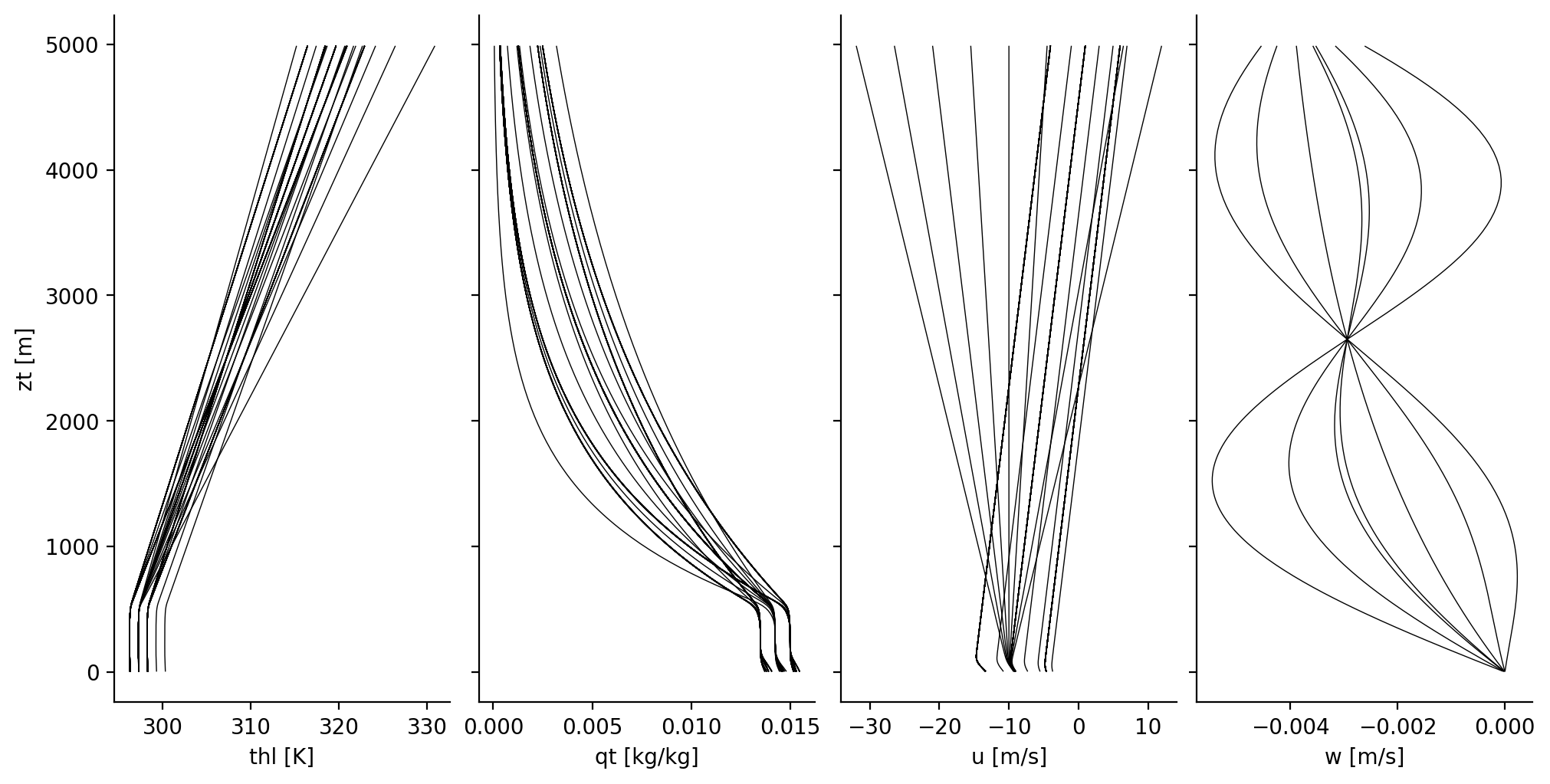
An overview over the initial profiles of Botany#
# Profiles of vertical velocity, from variations in first-mode amplitude
def expsinw(z, ampwp, w0=0.0045, Hw=2500, Hwp=5300):
    '''
    Vertical profiles for imposed, large-scale subsidence velocity
    '''
    w_0 = -w0*(1-np.exp(-z/Hw))
    w_1 = ampwp*np.sin(2.*np.pi/Hwp*z)
    w_1[z>Hwp] = 0.
    return w_0 + w_1

wpamp = np.unique(pd.DataFrame.from_records(parameters)[['wpamp']].to_numpy())

ds_initial = ds_profiles.isel(time=0).sel(zt=slice(0, 5000))

kws = {'y'          : 'zt',
       'add_legend' : False,
       'linewidth'  : 0.5,
       'c'          : 'k'}

fig, axs = plt.subplots(ncols=4, sharey=True, figsize=(10,5))

ds_initial['thl'].plot.line(ax=axs[0], **kws)
ds_initial['qt'].plot.line(ax=axs[1], **kws)
ds_initial['u'].plot.line(ax=axs[2], **kws)

for i, wpampi in enumerate(wpamp):
    axs[3].plot(expsinw(ds_initial['zt'], wpampi), ds_initial['zt'], linewidth=0.5, c='k')
axs[3].set_xlabel('w [m/s]')

for i in range(axs.size):
    axs[i].set_title('')
    if i > 0:
        axs[i].set_ylabel('')

plt.show()
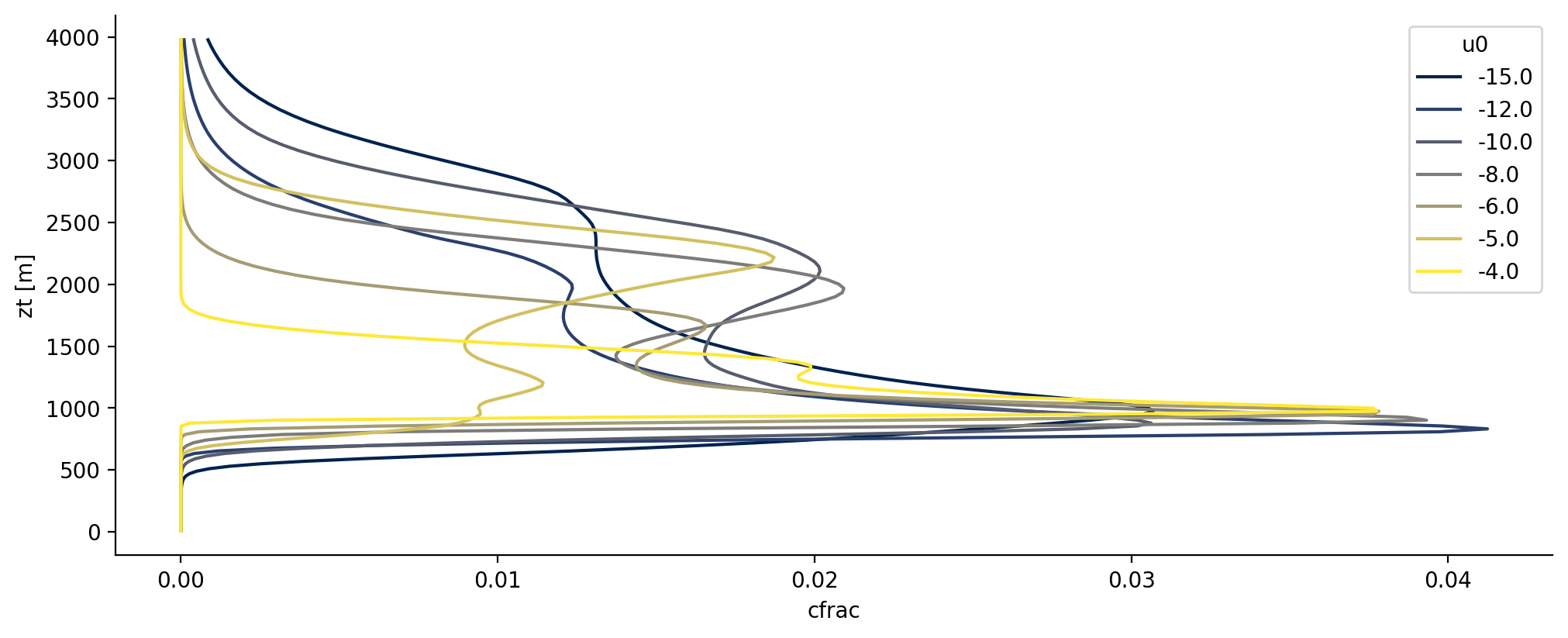
Variability of cloud fraction with surface wind#
One way to study how simulation output varies with the parameters is to add a variable of interest to one’s loaded xarray.Dataset:
from cycler import cycler

fig = plt.figure()
ax = plt.gca()
ax.set_prop_cycle(cycler(color=plt.cm.cividis(np.linspace(0, 1, 7))))

# Add u0 to the profiles output
ds_u = ds_profiles.assign(df_parameters[['member','u0']].set_index('member').to_xarray())

# Plot mean cloud fraction profiles grouped by surface wind over the last 100 time steps of all simulations
ds_u[['cfrac','u0']].isel(time=slice(-100,-1)).sel(zt = slice(0,4000)).mean(dim='time').groupby('u0').mean()['cfrac'].plot.line(ax=ax, y='zt')
plt.show()
/home/runner/miniconda3/envs/how_to_eurec4a/lib/python3.13/site-packages/xarray/core/dataset.py:4789: UserWarning: No index created for dimension u0 because variable u0 is not a coordinate. To create an index for u0, please first call `.set_coords('u0')` on this object.
  warnings.warn(
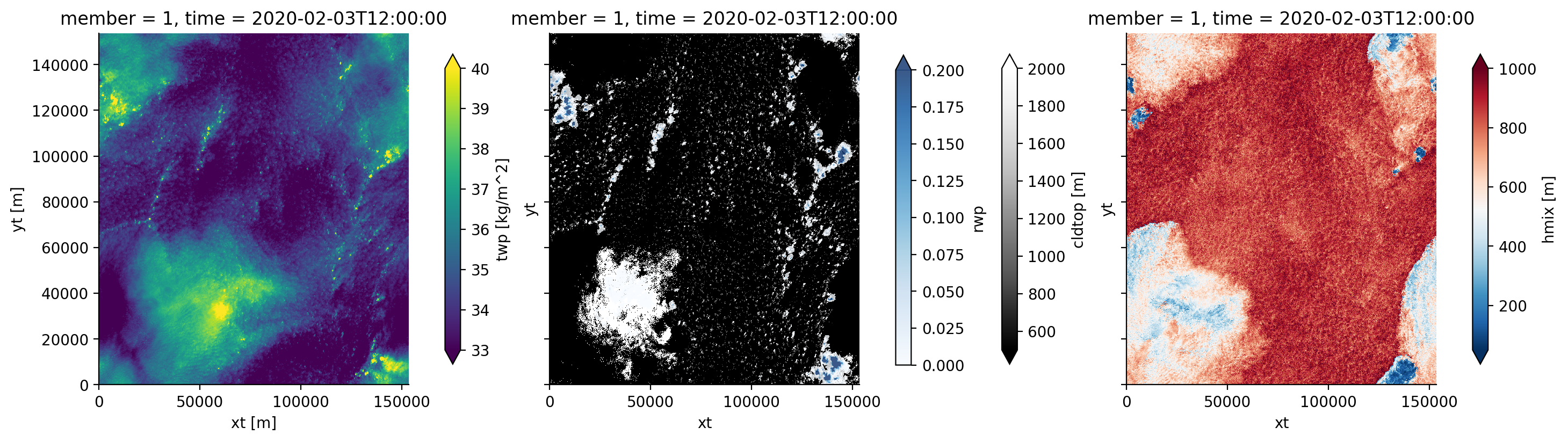
Example visualisation of water vapour, clouds, rain and cold pools#
For the last time (60 hours after initialisation) for the “center” of the hypercube of simulations (member 1), we might visualise the vertically integrated total specific humidity (the total water path twp), the cloud-top height (cldtop), the rain-water path (rwp) and an indicator for the extent of cold pools (the local mixed-layer height, hmix), as follows:
cb_kw = {'fraction' : 0.05}

ds_2D = botany_cat.dx100m.nx1536['2D'].to_dask().sel(member=1).isel(time=-1)
ds_2D
fig, axs = plt.subplots(ncols=3, sharex=True, sharey=True, figsize=(14.5,4))

# Total water path
ds_2D['twp'].plot(ax=axs[0], vmin=33 ,vmax=40, cbar_kwargs=cb_kw)

# Cloud-top height and rain water path
ds_2D['cldtop'].plot(ax=axs[1],cmap='Greys_r', vmin=500, vmax=2000, cbar_kwargs=cb_kw)
rwp_masked = xr.where(ds_2D['rwp'] > 1e-5, ds_2D['rwp'], np.nan)
rwp_masked.plot(ax=axs[1], cmap='Blues', vmin=0, vmax=0.2, alpha=0.8, cbar_kwargs=cb_kw)

# Mixed-layer height
ds_2D['hmix'].plot(ax=axs[2],cmap='RdBu_r', vmin=50, vmax=1000, cbar_kwargs=cb_kw)

plt.show()
/home/runner/miniconda3/envs/how_to_eurec4a/lib/python3.13/site-packages/intake_xarray/base.py:21: FutureWarning: The return type of `Dataset.dims` will be changed to return a set of dimension names in future, in order to be more consistent with `DataArray.dims`. To access a mapping from dimension names to lengths, please use `Dataset.sizes`.
  'dims': dict(self._ds.dims),
Visualisations page#
In addition to the data sets described above, a more thorough set of visualisations indicative simulation output is available. This visualisation set contains simple overviews and movies for each simulation in the library. They can be quite useful for attaining a basic idea of what each simulation produced without having to load the data. These visualisations are hosted on a personal server. Since the maintenance and availability of this server may be patchy, they can also be downloaded from Zenodo.