VELOX

Video airbornE Longwave Observations within siX channels

VELOX is a thermal infrared spectral imager (VELOX327k veL, 640 pixel by 512 pixels) with a synchronized filter wheel (at 100 Hz) covering six spectral channels in the thermal infrared wavelength range from 7.7 to 12.0 micrometer. The instrument measures the brightness temperature of upward radiance in a field-of-view of 35.49° by 28.71°.

The PI during EUREC⁴A was Michael Schäfer (University Leipzig).

If you have questions or if you would like to use the data for a publication, please don’t hesitate to get in contact with the dataset authors as stated in the dataset attributes contact or author.

Note

No data available for the transfer flights (first and last) and the first local research flight.

Get data

To load the data we first load the EUREC⁴A intake catalog and list the available datasets from VELOX. Currently, there is a cloud mask product available.

import eurec4a
cat = eurec4a.get_intake_catalog(use_ipfs="QmahMN2wgPauHYkkiTGoG2TpPBmj3p5FoYJAq9uE9iXT9N")
list(cat.HALO.VELOX)

['cloudmask']

ds = cat.HALO.VELOX.cloudmask["HALO-0205"].to_dask()
ds

/usr/share/miniconda3/envs/how_to_eurec4a/lib/python3.12/site-packages/intake_xarray/base.py:21: FutureWarning: The return type of `Dataset.dims` will be changed to return a set of dimension names in future, in order to be more consistent with `DataArray.dims`. To access a mapping from dimension names to lengths, please use `Dataset.sizes`.
  'dims': dict(self._ds.dims),

<xarray.Dataset> Size: 10GB
Dimensions:     (time: 29894, y: 512, x: 640)
Coordinates:
    alt         (time) float32 120kB dask.array<chunksize=(29894,), meta=np.ndarray>
    lat         (time) float32 120kB dask.array<chunksize=(29894,), meta=np.ndarray>
    lon         (time) float32 120kB dask.array<chunksize=(29894,), meta=np.ndarray>
  * time        (time) datetime64[ns] 239kB 2020-02-05T09:21:46 ... 2020-02-0...
Dimensions without coordinates: y, x
Data variables:
    CF_max      (time) float32 120kB dask.array<chunksize=(29894,), meta=np.ndarray>
    CF_min      (time) float32 120kB dask.array<chunksize=(29894,), meta=np.ndarray>
    cloud_mask  (y, x, time) int8 10GB dask.array<chunksize=(32, 40, 3737), meta=np.ndarray>
    vaa         (y, x) float32 1MB dask.array<chunksize=(256, 320), meta=np.ndarray>
    vza         (y, x) float32 1MB dask.array<chunksize=(256, 320), meta=np.ndarray>
Attributes: (12/22)
    Conventions:          "CF-1.8"
    author:               Michael Schäfer, André Ehrlich, Anna Luebke, Jakob ...
    campaign:             EUREC4A
    comment_1:            The cloud mask is derived with 1 Hz temporal resolu...
    comment_2:            Four different thresholds (0.5 K, 1.0 K, 1.5 K, and...
    comment_3:            The final cloud mask logically combines the differe...
    ...                   ...
    platform:             HALO
    research_flight_day:  20200205
    source:               Airborne imaging with the VELOX system
    title:                Two-dimensional cloud mask and cloud fraction with ...
    variable:             cloud_mask, CF_min, CF_max
    version:              Version 3 from 2021-02-12

xarray.Dataset

• Dimensions:
  • time: 29894
  • y: 512
  • x: 640
• Coordinates: (4)
  • alt
    (time)
    float32
    dask.array<chunksize=(29894,), meta=np.ndarray>

    description :

    Platform altitude coordinate

    long_name :

    altitude

    units :

    m

    Array Chunk Bytes 116.77 kiB 116.77 kiB Shape (29894,) (29894,) Dask graph 1 chunks in 2 graph layers Data type float32 numpy.ndarray

  • lat
    (time)
    float32
    dask.array<chunksize=(29894,), meta=np.ndarray>

    description :

    Platform latitude coordinate

    long_name :

    latitude

    standard_name :

    latitude

    units :

    degrees_north

    Array Chunk Bytes 116.77 kiB 116.77 kiB Shape (29894,) (29894,) Dask graph 1 chunks in 2 graph layers Data type float32 numpy.ndarray

  • lon
    (time)
    float32
    dask.array<chunksize=(29894,), meta=np.ndarray>

    description :

    Platform longitude coordinate

    long_name :

    longitude

    standard_name :

    longitude

    units :

    degrees_east

    Array Chunk Bytes 116.77 kiB 116.77 kiB Shape (29894,) (29894,) Dask graph 1 chunks in 2 graph layers Data type float32 numpy.ndarray

  • time
    (time)
    datetime64[ns]
    2020-02-05T09:21:46 ... 2020-02-...

    long_name :

    time

    array(['2020-02-05T09:21:46.000000000', '2020-02-05T09:21:47.000000000',
           '2020-02-05T09:21:48.000000000', ..., '2020-02-05T18:08:26.000000000',
           '2020-02-05T18:08:27.000000000', '2020-02-05T18:08:28.000000000'],
          dtype='datetime64[ns]')

• Data variables: (5)
  • CF_max
    (time)
    float32
    dask.array<chunksize=(29894,), meta=np.ndarray>

    description :

    Maximal possible cloud fraction derived from the ratio between the number of pixels classified with cloud mask values of "1b" and "2b" and the total number of usable pixels in the image.

    long_name :

    Maximal cloud fraction

    Array Chunk Bytes 116.77 kiB 116.77 kiB Shape (29894,) (29894,) Dask graph 1 chunks in 2 graph layers Data type float32 numpy.ndarray

  • CF_min
    (time)
    float32
    dask.array<chunksize=(29894,), meta=np.ndarray>

    description :

    Minimal possible cloud fraction derived from the ratio between the number of pixels classified with a cloud mask value of "2b" and the total number of usable pixels in the image.

    long_name :

    Minimal cloud fraction

    Array Chunk Bytes 116.77 kiB 116.77 kiB Shape (29894,) (29894,) Dask graph 1 chunks in 2 graph layers Data type float32 numpy.ndarray

  • cloud_mask
    (y, x, time)
    int8
    dask.array<chunksize=(32, 40, 3737), meta=np.ndarray>

    description :

    Cloud mask derived by comparing the measured brightness temperature with the brightness temperature in a clear-sky assumption using the four thresholds of 0.5 K, 1.0 K, 1.5 K, and 2.0 K. If all thresholds are exceeded, the measurement is denoted as "most_likely_cloudy", if only one of the thresholds is exceeded, the measurement is denoted as "probably_cloudy". "cloud_free" is classified when no threshold is reached. "unknown" is classified when no estimation of the cloud mask was possible, e.g. due to condensation on the window.

    flag_meanings :

    unknown cloud_free probably_cloudy most_likely_cloudy

    flag_values :

    [-1, 0, 1, 2]

    long_name :

    cloud flag

    Array Chunk Bytes 9.12 GiB 4.56 MiB Shape (512, 640, 29894) (32, 40, 3737) Dask graph 2048 chunks in 2 graph layers Data type int8 numpy.ndarray

  • vaa
    (y, x)
    float32
    dask.array<chunksize=(256, 320), meta=np.ndarray>

    description :

    Camera viewing azimuth angle of each spatial pixel, mathematic negative system with 0° into flight direction, clockwise.

    long_name :

    Viewing sensor azimuth angle

    units :

    degree

    Array Chunk Bytes 1.25 MiB 320.00 kiB Shape (512, 640) (256, 320) Dask graph 4 chunks in 2 graph layers Data type float32 numpy.ndarray

  • vza
    (y, x)
    float32
    dask.array<chunksize=(256, 320), meta=np.ndarray>

    description :

    Angle between the line of sight and the viewing direction of each spatial pixel of the sensor.

    long_name :

    Viewing sensor zenith angle

    units :

    degree

    Array Chunk Bytes 1.25 MiB 320.00 kiB Shape (512, 640) (256, 320) Dask graph 4 chunks in 2 graph layers Data type float32 numpy.ndarray

• Indexes: (1)
  • time
    PandasIndex

    PandasIndex(DatetimeIndex(['2020-02-05 09:21:46', '2020-02-05 09:21:47',
                   '2020-02-05 09:21:48', '2020-02-05 09:21:49',
                   '2020-02-05 09:21:50', '2020-02-05 09:21:52',
                   '2020-02-05 09:21:53', '2020-02-05 09:21:54',
                   '2020-02-05 09:22:05', '2020-02-05 09:22:06',
                   ...
                   '2020-02-05 18:08:19', '2020-02-05 18:08:20',
                   '2020-02-05 18:08:21', '2020-02-05 18:08:22',
                   '2020-02-05 18:08:23', '2020-02-05 18:08:24',
                   '2020-02-05 18:08:25', '2020-02-05 18:08:26',
                   '2020-02-05 18:08:27', '2020-02-05 18:08:28'],
                  dtype='datetime64[ns]', name='time', length=29894, freq=None))

• Attributes: (22)

  Conventions :

  "CF-1.8"

  author :

  Michael Schäfer, André Ehrlich, Anna Luebke, Jakob Thoböll, Kevin Wolf, Manfred Wendisch

  campaign :

  EUREC4A

  comment_1 :

  The cloud mask is derived with 1 Hz temporal resolution from the broadband channel of VELOX by comparing the measured brightness temperature with simulations assuming cloud-free conditions.

  comment_2 :

  Four different thresholds (0.5 K, 1.0 K, 1.5 K, and 2.0 K) for the difference between measurements and simulations are applied.

  comment_3 :

  The final cloud mask logically combines the different thresholds for each spatial pixel and each time step.

  comment_4 :

  If all thresholds are exceeded, the measurement is denoted as "most_likely_cloudy", if only one of the thresholds is exceeded, the measurement is denoted as "probably_cloudy". "cloud_free" is classified when no threshold is reached. "unknown" is classified when no estimation of the cloud mask was possible, e.g. due to condensation on the window.

  comment_5 :

  Due to possible condensation at the instrument window during the ascent, some data in the beginning of the flight might be not usable. Such data points are classified as "-1b, unknown".

  comment_6 :

  Flight direction is towards positive y-direction of the image

  comment_7 :

  Thermal infrared imager information: focal length: 15 mm, image size: 640 x 512 pixels, detector size: 9.60 mm x 7.68 mm, FOV: 35.49° x 28.71°

  contact_1 :

  Michael Schäfer, University Leipzig, michael.schaefer@uni-leipzig.de

  contact_2 :

  André Ehrlich, University Leipzig, a.ehrlich@uni-leipzig.de

  created_on :

  2021-02-12

  history :

  2021-02-06 flag_values, flag_meanings, and comments adapted to unified EUREC4A convention, 2021-02-12 vaa and vza included, descriptions updated, cloud_fraction as byte, alt lon lat source changed from SMART INS to BAHAMAS INS, minor changes

  institution :

  University of Leipzig, Leipzig Institute for Meteorology

  instrument :

  VELOX

  platform :

  HALO

  research_flight_day :

  20200205

  source :

  Airborne imaging with the VELOX system

  title :

  Two-dimensional cloud mask and cloud fraction with 1 Hz temporal resolution derived from VELOX during the EUREC4A field campaign.

  variable :

  cloud_mask, CF_min, CF_max

  version :

  Version 3 from 2021-02-12

What does the VELOX image look like at a specific dropsonde launch?

We can use the flight segmentation information to select a dropsonde and further extract the corresponding VELOX image taken at the time of the dropsonde launch.
In particular, we select the first dropsonde with the quality flag GOOD from the second circle on February 5.

Get dropsonde ID

(0) we read the meta data and extract the segment IDs

meta = eurec4a.get_flight_segments()

segments = [{**s,
             "platform_id": platform_id,
             "flight_id": flight_id
            }
            for platform_id, flights in meta.items()
            for flight_id, flight in flights.items()
            for s in flight["segments"]
           ]

(1) we extract the segment ID of the second circle

import datetime

segments_ordered_by_start_time = list(sorted(segments, key=lambda s: s["start"]))
circles_Feb05 = [s["segment_id"]
                 for s in segments_ordered_by_start_time
                 if "circle" in s["kinds"]
                 and s["start"].date() == datetime.date(2020,2,5)
                 and s["platform_id"] == "HALO"
                ]
second_circle_Feb05 = circles_Feb05[1]
second_circle_Feb05

'HALO-0205_c2'

(2) we extract the ID of the first dropsonde with flag GOOD in this circle

segments_by_segment_id = {s["segment_id"]: s for s in segments}
first_dropsonde = segments_by_segment_id[second_circle_Feb05]["dropsondes"]["GOOD"][0]
first_dropsonde

'HALO-0205_s13'

What is the corresponding launch time of the selected sonde?

So far, we only made use of the flight segmentation meta data. The launch time to a given sonde is stated in the JOANNE dataset (see also book chapter Dropsondes dataset JOANNE). We use again the intake catalog to load the JOANNE dataset and extract the launch time to the selected dropsonde by it’s sonde ID.

dropsondes = cat.dropsondes.JOANNE.level3.to_dask()

/usr/share/miniconda3/envs/how_to_eurec4a/lib/python3.12/site-packages/intake_xarray/base.py:21: FutureWarning: The return type of `Dataset.dims` will be changed to return a set of dimension names in future, in order to be more consistent with `DataArray.dims`. To access a mapping from dimension names to lengths, please use `Dataset.sizes`.
  'dims': dict(self._ds.dims),

sonde_dt = dropsondes.sel(sonde_id=first_dropsonde).launch_time.values
sonde_dt

numpy.datetime64('2020-02-05T10:47:46.000000000')

Cloud mask plot

Finally, we plot the VELOX image closest in time to the dropsonde launch.
The y-axis is in flight direction and the image consists of 640 pixel by 512 pixels. The corresponding pixel viewing sensor zenith and azimuth angles are given by the dataset variables vza and vaa.

ds_sel = ds.cloud_mask.sel(time=sonde_dt, method="nearest")

%matplotlib inline
import matplotlib.pyplot as plt
import pathlib
plt.style.use(pathlib.Path("./mplstyle/book"))

fig, ax = plt.subplots()

cax = ds_sel.plot(ax=ax,
                  cmap=plt.get_cmap('Greys', lut=4),
                  vmin=-1.5, vmax=2.5,
                  add_colorbar=False
                  )
cbar = fig.colorbar(cax, ticks=ds.cloud_mask.flag_values)
cbar.ax.set_yticklabels(ds.cloud_mask.flag_meanings.split(" "));

ax.set_title(f"VELOX cloud mask at {sonde_dt}");

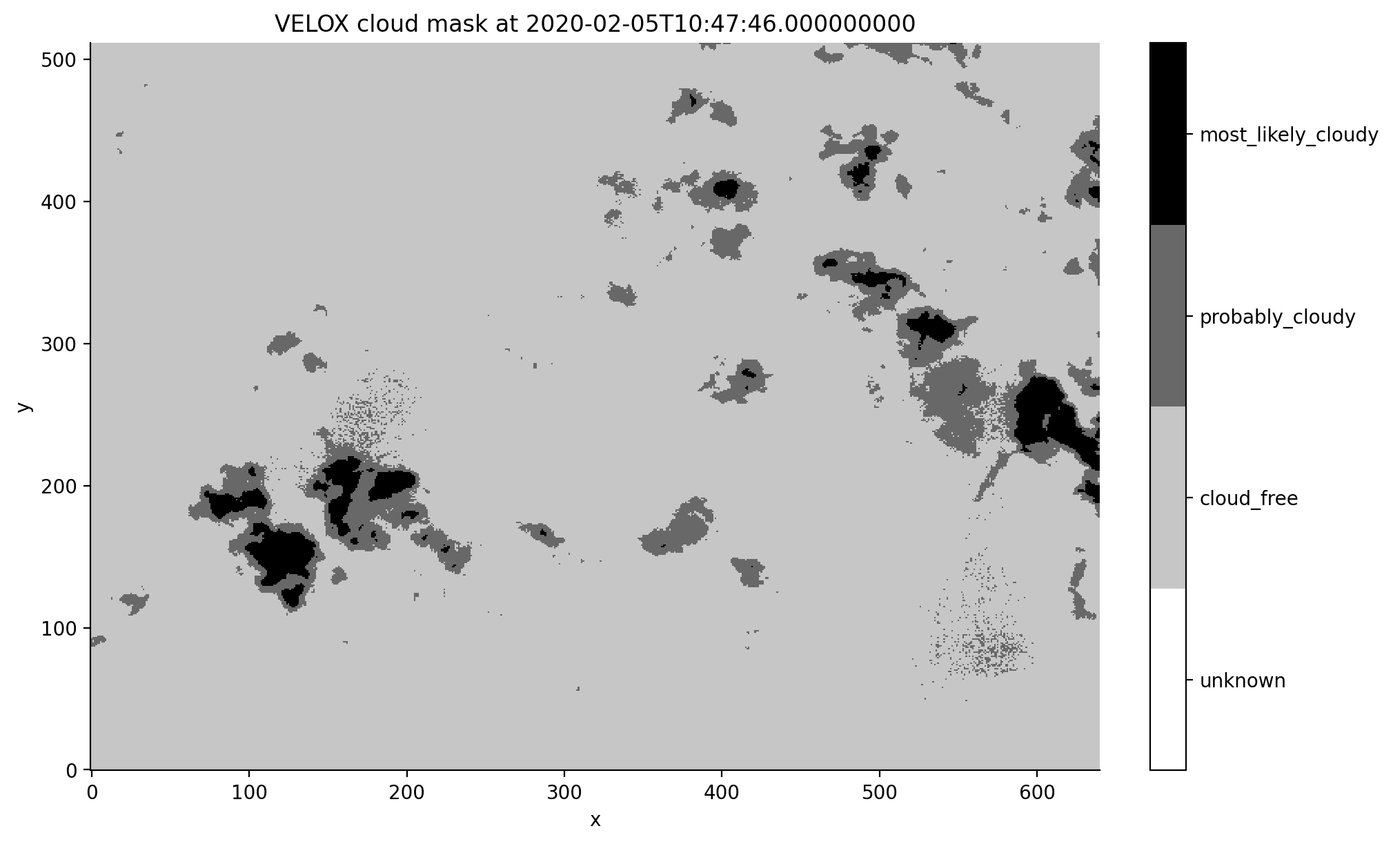
What are the image cloud fraction lower and upper bounds?

cfmin = ds.CF_min.sel(time=sonde_dt, method="nearest").values
cfmax = ds.CF_max.sel(time=sonde_dt, method="nearest").values
print(f"Image minimum cloud fraction (most likely cloudy): {cfmin:.2f}")
print(f"Image maximum cloud fraction (most likely and probably cloudy) :{cfmax:.2f}")

Image minimum cloud fraction (most likely cloudy): 0.02
Image maximum cloud fraction (most likely and probably cloudy) :0.09

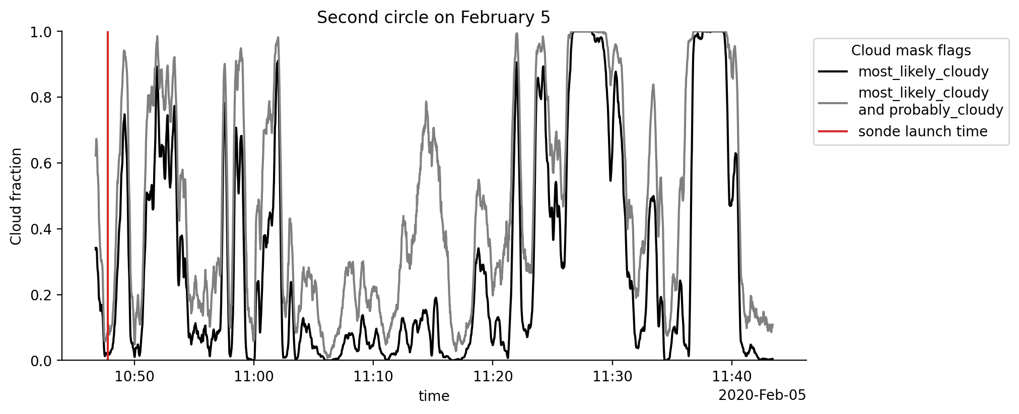
Cloud fraction time series from the second circle on February 5

We also want to show a time series of cloud fraction and use the segment ID from the second circle to extract and save the segment information to the variable seg. We can later use the segments start and end times to select the data in time.

seg = segments_by_segment_id[second_circle_Feb05]

The dataset variable CF_min provides a lower bound to cloud fraction estimates based on the cloud mask flag most_likely_cloudy, while CF_max provides an upper bound by including the uncertain pixels labeled probably cloudy.

selection = ds.sel(time=slice(seg["start"], seg["end"]))

with plt.style.context("mplstyle/wide"):
    fig, ax = plt.subplots()
    selection.CF_min.plot(color="k", label="most_likely_cloudy")
    selection.CF_max.plot(color="grey", label="most_likely_cloudy\nand probably_cloudy")
    ax.axvline(sonde_dt, color="C3", label="sonde launch time")
    ax.set_ylim(0, 1)
    ax.set_ylabel("Cloud fraction")
    ax.set_title("Second circle on February 5")
    ax.legend(title="Cloud mask flags", bbox_to_anchor=(1,1), loc="upper left");