Cloud radar data collected at the Barbados Cloud Observatory (BCO)

General information

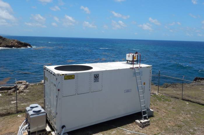
The polarised 35.5 GHz Doppler radar is part of the Combined Radar And Lidar instrument (CORAL) at the Barbados Cloud Observatory (BCO). It has a sensitivity of -48 dBZ at an altitude of 5 km and -70 dBZ at an altitude of 500 m. The radar has a range gating of 31.18 m and measures at ranges between 150 m and 18.9 km. It operates in a zenith looking mode, so that range gating effectively measures distance in the vertical. To measure the vertical velocity the radar uses the Doppler technique with an FFT of 256 samples, giving it a Doppler resolution of < 0.02 ms\(^{-1}\) between -10 and 10 ms\(^{-1}\). The radar is able to provide the linear depolarisation ratio (LDR), which can be used for a target classification based on their shape. Data processing and radar calibration are done by following Görsdorf et al. (2015), which leads to an uncertainty of 1.3 dB.

Radar characteristics

Characteristic	CORAL Ka-band radar
Radar type	Mono static, pulsed, magnetron
Frequency	35.5 GHz \(\pm\) 150 MHz
Peak power	30 kW
Pulse width	200 ns for 30 m range resolution
Doppler velocity resolution	0.02 ms\(^{-1}\)
Diameter of antenna	2 m
Antenna beam width	0.3 deg x 0.3 deg
Sensitivity	-48 dBZ at 5 km, -70 dBZ at 500 m

Getting the data catalog

The python code below allows you to analyze the available measurements within January/February 2020.

from datetime import datetime
import matplotlib.pyplot as plt
import pathlib
plt.style.use([pathlib.Path("./mplstyle/book"), pathlib.Path("./mplstyle/wide")])
import numpy as np
import eurec4a
cat = eurec4a.get_intake_catalog()

Getting the data from the BCO Ka-band radar

To get a list of BCO datasets that are available within the catalog, type:

list(cat['barbados.bco'])

['CORAL_LIDAR',
 'ceilometer',
 'POLDIRAD',
 'radar_reflectivity',
 'meteorology',
 'radiation',
 'MRR',
 'isotopes']

Loading the radar dataset

The entire radar dataset of the BCO Ka-band radar can be loaded lazy, i.e. only loading the metadata and not the data such like radar reflectivity itself, by typing:

ds = cat.barbados.bco.radar_reflectivity.to_dask()

/usr/share/miniconda3/envs/how_to_eurec4a/lib/python3.12/site-packages/intake_xarray/base.py:21: FutureWarning: The return type of `Dataset.dims` will be changed to return a set of dimension names in future, in order to be more consistent with `DataArray.dims`. To access a mapping from dimension names to lengths, please use `Dataset.sizes`.
  'dims': dict(self._ds.dims),

The variables that this dataset contains can be shown by typing:

ds

<xarray.Dataset> Size: 70GB
Dimensions:     (time: 2037350, range: 605)
Coordinates:
  * range       (range) float64 5kB 155.9 187.1 218.2 ... 1.896e+04 1.899e+04
  * time        (time) datetime64[ns] 16MB 2020-01-12T16:19:26 ... 2020-02-29...
Data variables: (12/23)
    HSDco       (time, range) float32 5GB dask.array<chunksize=(63668, 19), meta=np.ndarray>
    HSDcx       (time, range) float32 5GB dask.array<chunksize=(63668, 19), meta=np.ndarray>
    LDR         (time, range) float32 5GB dask.array<chunksize=(63668, 19), meta=np.ndarray>
    LDRg        (time, range) float32 5GB dask.array<chunksize=(63668, 19), meta=np.ndarray>
    MeltHei     (time) float32 8MB dask.array<chunksize=(127335,), meta=np.ndarray>
    RMS         (time, range) float32 5GB dask.array<chunksize=(63668, 19), meta=np.ndarray>
    ...          ...
    longitude   (time) float64 16MB dask.array<chunksize=(63668,), meta=np.ndarray>
    mask        (time, range) int8 1GB dask.array<chunksize=(63668, 38), meta=np.ndarray>
    northangle  (time) float32 8MB dask.array<chunksize=(127335,), meta=np.ndarray>
    status      (time) float32 8MB dask.array<chunksize=(127335,), meta=np.ndarray>
    tpow        (time) float32 8MB dask.array<chunksize=(127335,), meta=np.ndarray>
    zenith      (time) float32 8MB dask.array<chunksize=(127335,), meta=np.ndarray>
Attributes: (12/16)
    Altitude:        11 m
    Conventions:     CF-1.7
    DOI:             10.25326/55
    contact_person:  Lutz Hirsch (lutz.hirsch@mpimet.mpg.de)
    created_with:    mmclx_to_netcdf_OOP.py with its last modification on Sat...
    creation_date:   Sun Mar  1 07:21:58 2020
    ...              ...
    python_version:  3.6.9 |Anaconda, Inc.| (default, Jul 30 2019, 19:07:31) ...
    reference:       Ka Band Cloud Radar MIRA-3x, METEK GmbH www.metek.de
    source:          /pool/OBS/BARBADOS_CLOUD_OBSERVATORY/Level_1/B_Reflectiv...
    system:          MIRA36
    title:           MIRA-3x Cloud Radar Data
    version:         1.1.1-434-g3e3deca

xarray.Dataset

• Dimensions:
  • time: 2037350
  • range: 605
• Coordinates: (2)
  • range
    (range)
    float64
    155.9 187.1 ... 1.896e+04 1.899e+04

    axis :

    Z

    long_name :

    range from antenna to the center of each range gate

    standard_name :

    height

    units :

    m

    array([  155.9 ,   187.08,   218.25, ..., 18925.78, 18956.95, 18988.13])

  • time
    (time)
    datetime64[ns]
    2020-01-12T16:19:26 ... 2020-02-...

    axis :

    T

    standard_name :

    time

    array(['2020-01-12T16:19:26.000000000', '2020-01-12T16:19:28.000000000',
           '2020-01-12T16:19:30.000000000', ..., '2020-02-29T23:59:53.000000000',
           '2020-02-29T23:59:55.000000000', '2020-02-29T23:59:57.000000000'],
          dtype='datetime64[ns]')

• Data variables: (23)
  • HSDco
    (time, range)
    float32
    dask.array<chunksize=(63668, 19), meta=np.ndarray>

    db :

    1

    long_name :

    co-channel HSdiv noise power. The arbitrary unit is DSP.

    units :

    1

    valid_range :

    [-20.0, 40.0]

    Array Chunk Bytes 4.59 GiB 4.61 MiB Shape (2037350, 605) (63668, 19) Dask graph 1024 chunks in 2 graph layers Data type float32 numpy.ndarray

  • HSDcx
    (time, range)
    float32
    dask.array<chunksize=(63668, 19), meta=np.ndarray>

    db :

    1

    long_name :

    cross-channel HSdiv noise power. The arbitrary unit is DSP.

    units :

    1

    valid_range :

    [-20.0, 40.0]

    Array Chunk Bytes 4.59 GiB 4.61 MiB Shape (2037350, 605) (63668, 19) Dask graph 1024 chunks in 2 graph layers Data type float32 numpy.ndarray

  • LDR
    (time, range)
    float32
    dask.array<chunksize=(63668, 19), meta=np.ndarray>

    long_name :

    linear de-polarization ratio LDR of all hydrometeors

    units :

    dBZ

    Array Chunk Bytes 4.59 GiB 4.61 MiB Shape (2037350, 605) (63668, 19) Dask graph 1024 chunks in 2 graph layers Data type float32 numpy.ndarray

  • LDRg
    (time, range)
    float32
    dask.array<chunksize=(63668, 19), meta=np.ndarray>

    long_name :

    linear de-polarization ratio LDR of all targets (global)

    units :

    dBZ

    Array Chunk Bytes 4.59 GiB 4.61 MiB Shape (2037350, 605) (63668, 19) Dask graph 1024 chunks in 2 graph layers Data type float32 numpy.ndarray

  • MeltHei
    (time)
    float32
    dask.array<chunksize=(127335,), meta=np.ndarray>

    db :

    0

    long_name :

    melting layer height

    units :

    m

    valid_range :

    [0, 14000]

    Array Chunk Bytes 7.77 MiB 497.40 kiB Shape (2037350,) (127335,) Dask graph 16 chunks in 2 graph layers Data type float32 numpy.ndarray

  • RMS
    (time, range)
    float32
    dask.array<chunksize=(63668, 19), meta=np.ndarray>

    db :

    0

    long_name :

    peak width RMS of all hydrometeors

    units :

    m s-1

    valid_range :

    [0.0, 3.0]

    Array Chunk Bytes 4.59 GiB 4.61 MiB Shape (2037350, 605) (63668, 19) Dask graph 1024 chunks in 2 graph layers Data type float32 numpy.ndarray

  • RMSg
    (time, range)
    float32
    dask.array<chunksize=(63668, 19), meta=np.ndarray>

    db :

    0

    long_name :

    peak width RMS of all targets (global)

    units :

    m s-1

    valid_range :

    [0.0, 3.0]

    Array Chunk Bytes 4.59 GiB 4.61 MiB Shape (2037350, 605) (63668, 19) Dask graph 1024 chunks in 2 graph layers Data type float32 numpy.ndarray

  • RadarConst
    (time)
    float32
    dask.array<chunksize=(127335,), meta=np.ndarray>

    db :

    1

    long_name :

    radar constant related to 5 km height

    units :

    mm6 m-3

    valid_range :

    [-35.0, -20.0]

    Array Chunk Bytes 7.77 MiB 497.40 kiB Shape (2037350,) (127335,) Dask graph 16 chunks in 2 graph layers Data type float32 numpy.ndarray

  • SNR
    (time, range)
    float32
    dask.array<chunksize=(63668, 19), meta=np.ndarray>

    long_name :

    reflectivity SNR

    units :

    dBZ

    Array Chunk Bytes 4.59 GiB 4.61 MiB Shape (2037350, 605) (63668, 19) Dask graph 1024 chunks in 2 graph layers Data type float32 numpy.ndarray

  • SNRg
    (time, range)
    float32
    dask.array<chunksize=(63668, 19), meta=np.ndarray>

    long_name :

    reflectivity SNRg

    units :

    dBZ

    Array Chunk Bytes 4.59 GiB 4.61 MiB Shape (2037350, 605) (63668, 19) Dask graph 1024 chunks in 2 graph layers Data type float32 numpy.ndarray

  • SNRplank
    (time, range)
    float32
    dask.array<chunksize=(63668, 19), meta=np.ndarray>

    long_name :

    reflectivity SNRplank

    units :

    dBZ

    Array Chunk Bytes 4.59 GiB 4.61 MiB Shape (2037350, 605) (63668, 19) Dask graph 1024 chunks in 2 graph layers Data type float32 numpy.ndarray

  • VEL
    (time, range)
    float32
    dask.array<chunksize=(63668, 19), meta=np.ndarray>

    db :

    0

    long_name :

    doppler velocity VEL of all hydrometeors

    units :

    m s-1

    valid_range :

    [-10.661450386047363, 10.661450386047363]

    Array Chunk Bytes 4.59 GiB 4.61 MiB Shape (2037350, 605) (63668, 19) Dask graph 1024 chunks in 2 graph layers Data type float32 numpy.ndarray

  • VELg
    (time, range)
    float32
    dask.array<chunksize=(63668, 19), meta=np.ndarray>

    db :

    0

    long_name :

    doppler velocity VEL of all targets (global)

    units :

    m s-1

    valid_range :

    [-10.661450386047363, 10.661450386047363]

    Array Chunk Bytes 4.59 GiB 4.61 MiB Shape (2037350, 605) (63668, 19) Dask graph 1024 chunks in 2 graph layers Data type float32 numpy.ndarray

  • Ze
    (time, range)
    float32
    dask.array<chunksize=(63668, 19), meta=np.ndarray>

    long_name :

    equivalent radar reflectivity of all hydrometeors

    units :

    dBZ

    Array Chunk Bytes 4.59 GiB 4.61 MiB Shape (2037350, 605) (63668, 19) Dask graph 1024 chunks in 2 graph layers Data type float32 numpy.ndarray

  • Zf
    (time, range)
    float32
    dask.array<chunksize=(63668, 19), meta=np.ndarray>

    applied_thresholds :

    dBZ < -35 and VELg < -2.0 or VELg > 0.5 between 1000m and 8000m

    details :

    artifacts (rabbit-ears), caused by side lobes, are removed

    long_name :

    rabbit-ear filtered radar reflectivity of all hydrometeors

    standard_name :

    equivalent_reflectivity_factor

    units :

    dBZ

    Array Chunk Bytes 4.59 GiB 4.61 MiB Shape (2037350, 605) (63668, 19) Dask graph 1024 chunks in 2 graph layers Data type float32 numpy.ndarray

  • Zg
    (time, range)
    float32
    dask.array<chunksize=(63668, 19), meta=np.ndarray>

    long_name :

    equivalent radar reflectivity of all targets (global)

    units :

    dBZ

    Array Chunk Bytes 4.59 GiB 4.61 MiB Shape (2037350, 605) (63668, 19) Dask graph 1024 chunks in 2 graph layers Data type float32 numpy.ndarray

  • latitude
    (time)
    float64
    dask.array<chunksize=(63668,), meta=np.ndarray>

    long_name :

    north latitude

    units :

    degree_north

    valid_max :

    90.0

    valid_min :

    -90.0

    Array Chunk Bytes 15.54 MiB 497.41 kiB Shape (2037350,) (63668,) Dask graph 32 chunks in 2 graph layers Data type float64 numpy.ndarray

  • longitude
    (time)
    float64
    dask.array<chunksize=(63668,), meta=np.ndarray>

    long_name :

    east longitude

    units :

    degree_east

    valid_max :

    180.0

    valid_min :

    -180.0

    Array Chunk Bytes 15.54 MiB 497.41 kiB Shape (2037350,) (63668,) Dask graph 32 chunks in 2 graph layers Data type float64 numpy.ndarray

  • mask
    (time, range)
    int8
    dask.array<chunksize=(63668, 38), meta=np.ndarray>

    flag_meanings :

    rabbit_ear_retrieval no_rabbit_ear_retrieval

    flag_values :

    False True

    long_name :

    rabbit ear mask

    units :

    1

    usage :

    multiply radar products with this mask to reduce false signals by rabbit-ear retrievals

    Array Chunk Bytes 1.15 GiB 2.31 MiB Shape (2037350, 605) (63668, 38) Dask graph 512 chunks in 2 graph layers Data type int8 numpy.ndarray

  • northangle
    (time)
    float32
    dask.array<chunksize=(127335,), meta=np.ndarray>

    long_name :

    north angle

    units :

    degree

    Array Chunk Bytes 7.77 MiB 497.40 kiB Shape (2037350,) (127335,) Dask graph 16 chunks in 2 graph layers Data type float32 numpy.ndarray

  • status
    (time)
    float32
    dask.array<chunksize=(127335,), meta=np.ndarray>

    flag_meanings :

    radar_off radar_on

    flag_values :

    0 1

    long_name :

    radar power flag

    units :

    1

    Array Chunk Bytes 7.77 MiB 497.40 kiB Shape (2037350,) (127335,) Dask graph 16 chunks in 2 graph layers Data type float32 numpy.ndarray

  • tpow
    (time)
    float32
    dask.array<chunksize=(127335,), meta=np.ndarray>

    long_name :

    average transmit power

    units :

    W

    Array Chunk Bytes 7.77 MiB 497.40 kiB Shape (2037350,) (127335,) Dask graph 16 chunks in 2 graph layers Data type float32 numpy.ndarray

  • zenith
    (time)
    float32
    dask.array<chunksize=(127335,), meta=np.ndarray>

    long_name :

    zenith angle

    standard_name :

    sensor_zenith_angle

    units :

    degree

    Array Chunk Bytes 7.77 MiB 497.40 kiB Shape (2037350,) (127335,) Dask graph 16 chunks in 2 graph layers Data type float32 numpy.ndarray

• Indexes: (2)
  • range
    PandasIndex

    PandasIndex(Index([   155.9,   187.08,   218.25,   249.43,   280.61,   311.79,   342.97,
             374.15,   405.33,   436.51,
           ...
           18707.52,  18738.7, 18769.88, 18801.06, 18832.24, 18863.42,  18894.6,
           18925.78, 18956.95, 18988.13],
          dtype='float64', name='range', length=605))

  • time
    PandasIndex

    PandasIndex(DatetimeIndex(['2020-01-12 16:19:26', '2020-01-12 16:19:28',
                   '2020-01-12 16:19:30', '2020-01-12 16:19:32',
                   '2020-01-12 16:19:34', '2020-01-12 16:19:36',
                   '2020-01-12 16:19:38', '2020-01-12 16:19:40',
                   '2020-01-12 16:19:42', '2020-01-12 16:19:44',
                   ...
                   '2020-02-29 23:59:39', '2020-02-29 23:59:41',
                   '2020-02-29 23:59:43', '2020-02-29 23:59:45',
                   '2020-02-29 23:59:47', '2020-02-29 23:59:49',
                   '2020-02-29 23:59:51', '2020-02-29 23:59:53',
                   '2020-02-29 23:59:55', '2020-02-29 23:59:57'],
                  dtype='datetime64[ns]', name='time', length=2037350, freq=None))

• Attributes: (16)

  Altitude :

  11 m

  Conventions :

  CF-1.7

  DOI :

  10.25326/55

  contact_person :

  Lutz Hirsch (lutz.hirsch@mpimet.mpg.de)

  created_with :

  mmclx_to_netcdf_OOP.py with its last modification on Sat Nov 16 01:59:42 2019

  creation_date :

  Sun Mar 1 07:21:58 2020

  history :

  Concatenated dataset of daily converted source files

  institution :

  Max Planck Institute for Meteorology, Hamburg

  instrument :

  MBR2 cloud radar

  location :

  The Barbados Cloud Observatory, Deebles Point, Barbados, West Indies

  python_version :

  3.6.9 |Anaconda, Inc.| (default, Jul 30 2019, 19:07:31) [GCC 7.3.0] (with numpy version :1.15.4)

  reference :

  Ka Band Cloud Radar MIRA-3x, METEK GmbH www.metek.de

  source :

  /pool/OBS/BARBADOS_CLOUD_OBSERVATORY/Level_1/B_Reflectivity/Ka-Band/MBR2/2s/20200[12]/MMCR__MBR2__Spectral_Moments__2s__155m-18km__200[12]*.nc

  system :

  MIRA36

  title :

  MIRA-3x Cloud Radar Data

  version :

  1.1.1-434-g3e3deca

Plot some radar quantities

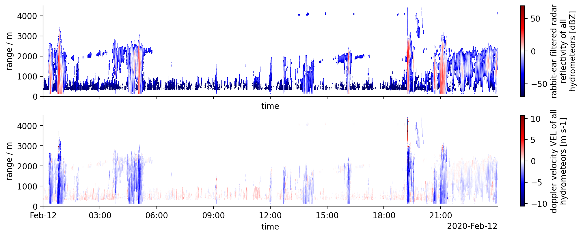
To create time/height plots for radar moments, pick a variable name having dimension (time, height) from the list of data variables and type the name in the code below. Common quantities that are used from the radar are radar reflectivity and doppler velocity. The radar reflectivity that is corrected for “rabbit ears” is saved in Zf.

In the following an example timeseries for both of these quantities is shown: to select the entire day :

time_min = np.datetime64('2020-02-12T00:00:00')
time_max = np.datetime64('2020-02-12T23:59:59')

# selecting subset of data
ds_sliced = ds.sel(time=slice(time_min, time_max))

fig, axs = plt.subplots(2,1, sharex=True)
# set here the variable from ds to plot, its color map and its min and max values
ds_sliced.Zf.plot(x='time', y='range', cmap="seismic", ax=axs[0])
ds_sliced.VEL.plot(x='time', y='range', cmap="seismic", ax=axs[1])
axs[1].set_xlim(time_min, time_max)
axs[0].set_ylim(0, 4500);
axs[1].set_ylim(0, 4500);
axs[0].set_ylabel('range / m')
axs[1].set_ylabel('range / m')

Text(0, 0.5, 'range / m')

Retrieving cloud fraction profile

The cloud fraction profile provides information about the variability of cloudiness at different height levels. The radar is often used to retrieve such a profile, but it should be noted that cloud quantities are not easy to define (see also the section about the HALO cloud mask product) and the cloud fraction profile can look very different depending on the instrument and its sensitivity. The Ka-Band radar at the BCO captures for example not only cloud and rain droplets, but also moistened sea-salt aerosols. The example below illustrates how the profiles depend on the chosen reflectivity threshold. Note, to be precise the following examples shows the echo fraction and not the cloud fraction.

fig, ax = plt.subplots(figsize=(2,3))
# calculate the mean cloud fraction profile
(~np.isnan(ds_sliced.Zf.sel(range=slice(0,4500)))).mean(dim='time').plot(y='range', label='no threshold')
# reduce sensitivity
threshold = -50
(ds_sliced.Zf > threshold).sel(range=slice(0,4500)).mean(dim='time').plot(y='range', label=f'{threshold} dBZ')
plt.title("Mean echo fraction")
plt.xlabel('echo fraction')
plt.legend();

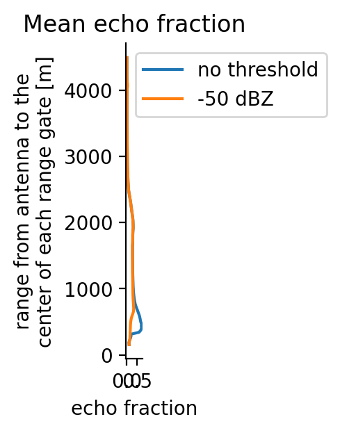
The threshold of -50 dBZ is chosen following Klingebiel et al. (2019) to exclude reflectivities from moistened sea-salt aerosols. For questions regarding the instrument, please contact the contact person given in the metadata of this dataset.