specMACS cloudmask#
The following script exemplifies the access and usage of specMACS data measured during EUREC⁴A.
The specMACS sensor consists of hyperspectral image sensors as well as polarization resolving image sensors.
The hyperspectral image sensors operate in the visible and near infrared (VNIR) and the short-wave infrared (SWIR) range.
The dataset investigated in this notebook is a cloud mask dataset based on data from the SWIR sensor.
More information on the dataset can be found on the macsServer. If you have questions or if you would like to use the data for a publication, please don’t hesitate to get in contact with the dataset authors as stated in the dataset attributes contact and author list.
Our plan is to analyze a section of the specMACS cloud mask dataset around the first GOOD dropsonde on the second HALO circle on the 5th of February (HALO-0205_c2). We’ll first look at the cloudiness just along the flight track and later on create a map projection of the dataset. This notebook will guide you through the required steps.
Obtaining data#
In order to work with EUREC⁴A datasets, we’ll use the eurec4a library to access the datasets and also use numpy and xarray as our common tools to handle datasets.
import eurec4a
import numpy as np
import xarray as xr
Finding the right sonde#
All HALO flights were split up into flight phases or segments to allow for a precise selection in time and space of a circle or calibration pattern. For more information have a look at the respective github repository.
all_flight_segments = eurec4a.get_flight_segments()
The flight segmentation data is organized by platform and flight, but as we want to look up a segment by its segment_id, we’ll have to flatten the data and reorganize it by the segment_id. Additionally, we want to be able to extract the flight_id and platform_id back from a selected segment, so we add this information to each individual segment:
segments_by_segment_id = {
    s["segment_id"]: {
        **s,
        "platform_id": platform_id,
        "flight_id": flight_id
    }
    for platform_id, flights in all_flight_segments.items()
    for flight_id, flight in flights.items()
    for s in flight["segments"]
}
We want to extract the id of the first dropsonde of the second HALO circle on February 5 (HALO-0205_c2). By the way: In the VELOX example the measurement of this time is shown as well.
segment = segments_by_segment_id["HALO-0205_c2"]
first_dropsonde = segment["dropsondes"]["GOOD"][0]
first_dropsonde
'HALO-0205_s13'
Now we would like to know when this sonde was launched. The JOANNE dataset contains this information. We use level 3 data which contains quality checked data on a common grid and load it using the intake catalog. We then select the correct dropsonde by its sonde_id to find out the launch time of the dropsonde.
More information on the data catalog can be found here.
cat = eurec4a.get_intake_catalog(use_ipfs="QmahMN2wgPauHYkkiTGoG2TpPBmj3p5FoYJAq9uE9iXT9N")
dropsondes = cat.dropsondes.JOANNE.level3.to_dask()
sonde_dt = dropsondes.sel(sonde_id=first_dropsonde).launch_time.values
str(sonde_dt)
/home/runner/miniconda3/envs/how_to_eurec4a/lib/python3.13/site-packages/intake_xarray/base.py:21: FutureWarning: The return type of `Dataset.dims` will be changed to return a set of dimension names in future, in order to be more consistent with `DataArray.dims`. To access a mapping from dimension names to lengths, please use `Dataset.sizes`.
  'dims': dict(self._ds.dims),
'2020-02-05T10:47:46.000000000'
Finding the corresponding specMACS dataset#
As specMACS data is organized as one dataset per flight, we have to obtain the flight_id from our selected segment to obtain the corresponding dataset. From this dataset, we select a two minute long measurement sequence of specMACS data around the dropsonde launch and have a look at the obtained dataset:
offset_time = np.timedelta64(60, "s")

ds = cat.HALO.specMACS.cloudmaskSWIR[segment["flight_id"]].to_dask()
ds_selection = ds.sel(time=slice(sonde_dt-offset_time, sonde_dt+offset_time))
ds_selection
/home/runner/miniconda3/envs/how_to_eurec4a/lib/python3.13/site-packages/intake_xarray/base.py:21: FutureWarning: The return type of `Dataset.dims` will be changed to return a set of dimension names in future, in order to be more consistent with `DataArray.dims`. To access a mapping from dimension names to lengths, please use `Dataset.sizes`.
  'dims': dict(self._ds.dims),
<xarray.Dataset> Size: 14MB
Dimensions:     (time: 3564, angle: 318)
Coordinates:
    alt         (time) float32 14kB dask.array<chunksize=(3564,), meta=np.ndarray>
  * angle       (angle) float64 3kB 18.0 17.9 17.8 ... -17.07 -17.17 -17.27
    lat         (time) float64 29kB dask.array<chunksize=(3564,), meta=np.ndarray>
    lon         (time) float64 29kB dask.array<chunksize=(3564,), meta=np.ndarray>
  * time        (time) datetime64[ns] 29kB 2020-02-05T10:46:46.015932928 ... ...
Data variables:
    CF_max      (time) float64 29kB dask.array<chunksize=(3564,), meta=np.ndarray>
    CF_min      (time) float64 29kB dask.array<chunksize=(3564,), meta=np.ndarray>
    cloud_mask  (time, angle) float32 5MB dask.array<chunksize=(3564, 20), meta=np.ndarray>
    vaa         (time, angle) float32 5MB dask.array<chunksize=(3564, 20), meta=np.ndarray>
    vza         (time, angle) float32 5MB dask.array<chunksize=(3564, 20), meta=np.ndarray>
Attributes: (12/15)
    Conventions:  CF-1.8
    author:       Veronika Pörtge, Felix Gödde, Tobias Kölling, Linda Forster...
    campaign:     EUREC4A
    comment:      The additional information about the viewing geometry and t...
    contact:      veronika.poertge@physik.uni-muenchen.de
    created_on:   2021-03-12
    ...           ...
    platform:     HALO
    references:   more information about the product can be found here: https...
    source:       airborne hyperspectral imaging with specMACS camera system
    title:        cloud mask derived from specMACS SWIR camera data captured ...
    variable:     cloud_mask
version: 2.1You can get a list of available variables in the dataset from ds_selection.variables.keys() or by looking them up in the table above.
First plots#
After selecting our datasets, we want to see what’s inside, so here are some first plots.
%matplotlib inline
import pathlib
import matplotlib.pyplot as plt
plt.style.use([pathlib.Path("./mplstyle/book"), pathlib.Path("./mplstyle/wide")])
First, we create a little helper to properly display a colorbar for categorical (in CF-Convention terms “flag”) variables:
def flagbar(fig, mappable, variable):
    ticks = variable.flag_values
    labels = variable.flag_meanings.split(" ")
    cbar = fig.colorbar(mappable, ticks=ticks)
    cbar.ax.set_yticklabels(labels);
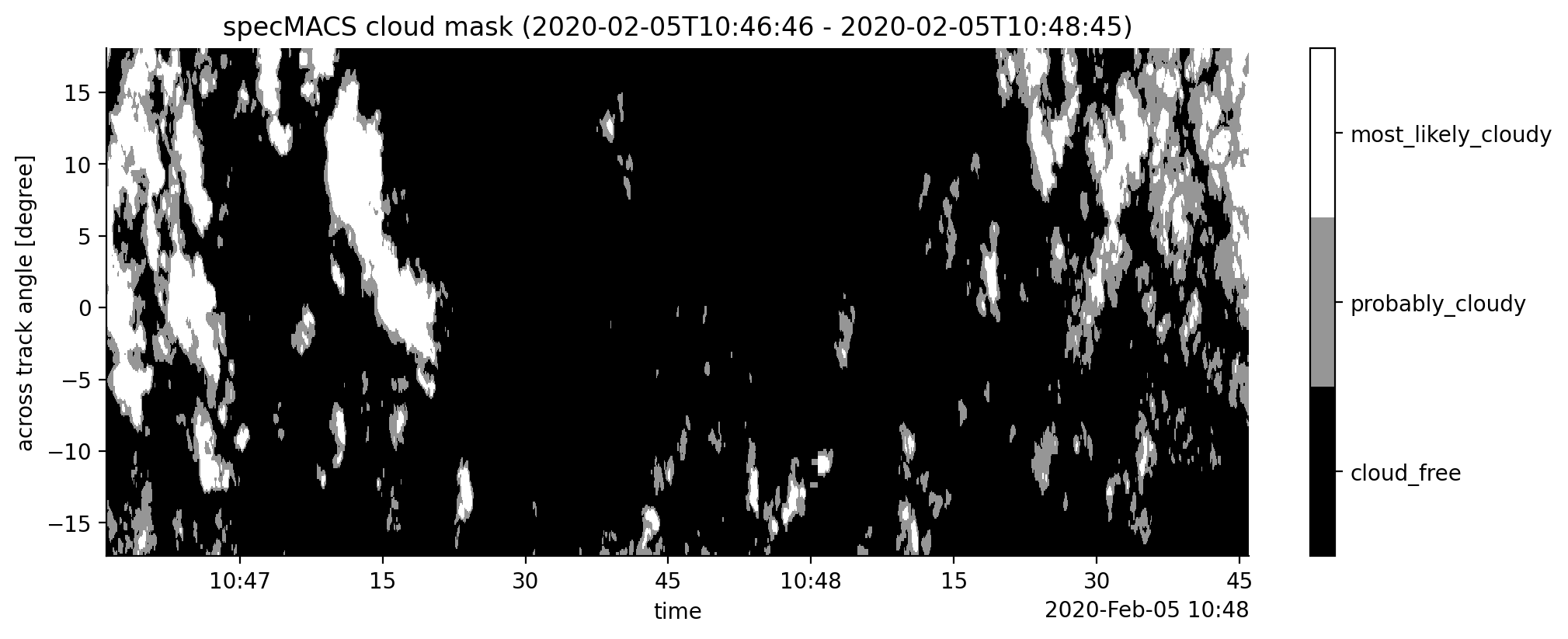
Figure 1: shows the SWIR camera cloud mask product along the flight track (x axis) for all observations in across track directions (y axis).
Note
fetching the data and displaying it might take a few seconds
fig, ax = plt.subplots()
cmplot = ds_selection.cloud_mask.T.plot(ax=ax,
                                        cmap=plt.get_cmap('Greys_r', lut=3),
                                        vmin=-0.5, vmax=2.5,
                                        add_colorbar=False)
flagbar(fig, cmplot, ds_selection.cloud_mask)
start_time_rounded, end_time_rounded = ds_selection.time.isel(time=[0, -1]).values.astype('datetime64[s]')
ax.set_title(f"specMACS cloud mask ({start_time_rounded} - {end_time_rounded})");
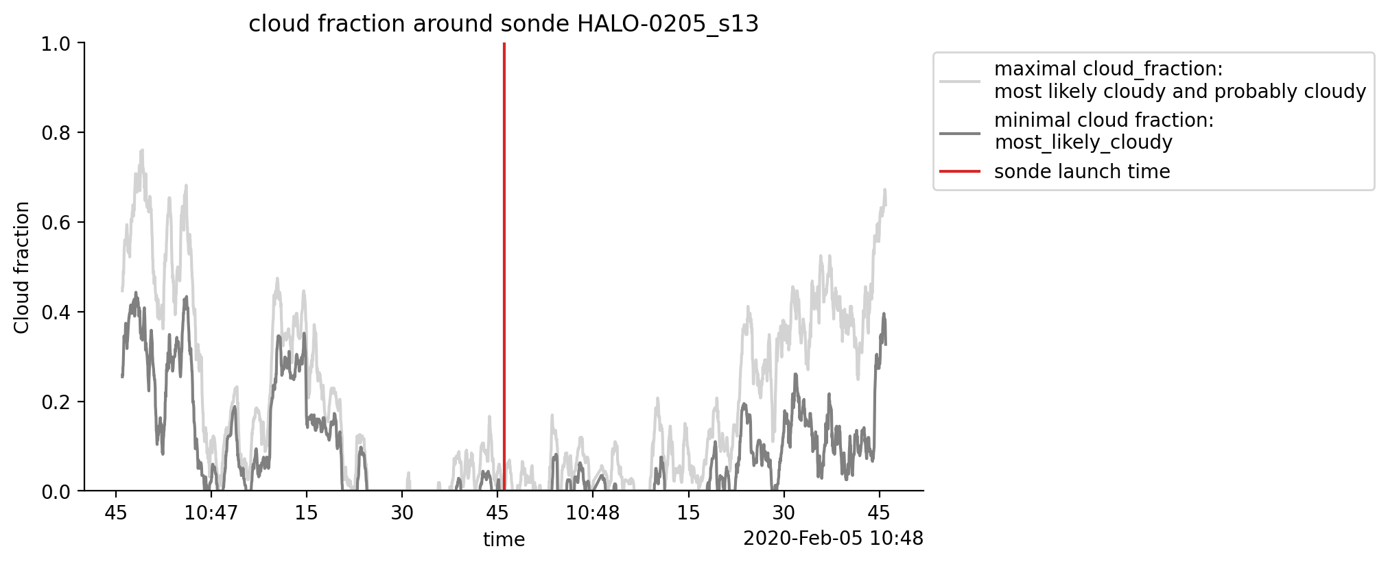
The dataset also contains the minimal and maximal cloud fractions which are calculated for each temporal measurement. The minimal cloud fraction is derived from the ratio between the number of pixels classified as “most likely cloudy” and the total number of pixels in one measurement (times with unknown measurements are excluded). The maximal cloud fraction additionally includes the number of pixels classified as “probably cloudy”.
fig, ax = plt.subplots()
ds_selection.CF_max.plot(color="lightgrey",label="maximal cloud_fraction:\nmost likely cloudy and probably cloudy")
ds_selection.CF_min.plot(color="grey", label="minimal cloud fraction:\nmost_likely_cloudy")
ax.axvline(sonde_dt, color="C3", label="sonde launch time")
ax.set_ylim(0, 1)
ax.set_ylabel("Cloud fraction")
ax.set_title(f"cloud fraction around sonde {first_dropsonde}")
ax.legend(bbox_to_anchor=(1,1), loc="upper left");
Camera view angles to latitude and longitude#
The cloud mask is given on a time \(\times\) angle grid where angles are the internal camera angles. Sometimes it could be helpful to project the data onto a map. This means that we would like to know the corresponding latitude and longitude coordinates of each pixel of the cloud mask.
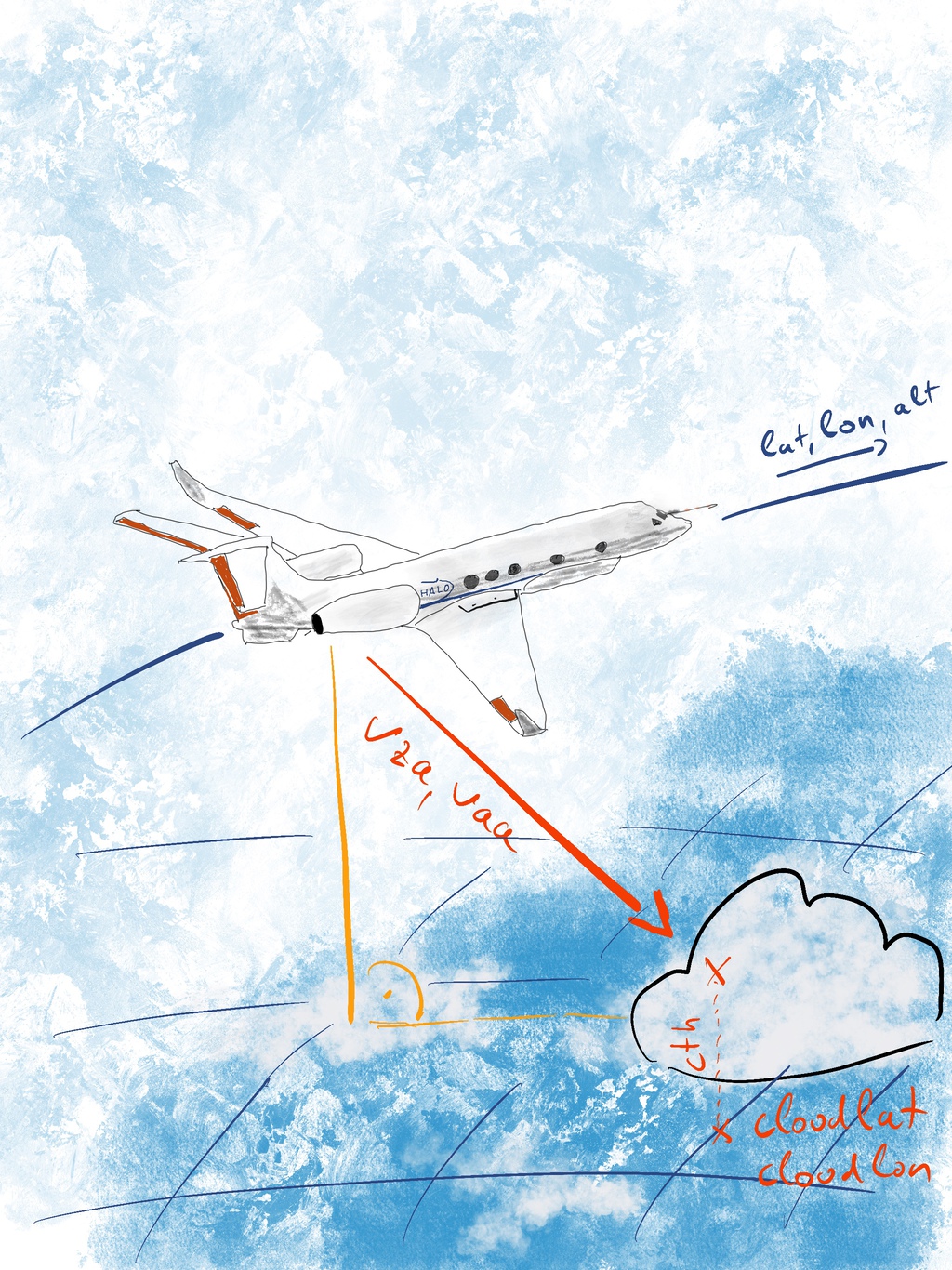
The computation involves quite a few steps, so let’s take a second to lay out a strategy. We know already the position of the aircraft and the individual viewing directions of each sensor pixel at each point in time. If we would start from the position of the aircraft and continue along each line of sight, until we hit something which we see in our dataset, we should end up at the location we are interested in. Due to the curvature of the earth, we’ll have to do a few coordinate transformations in the process, but no worries, we’ll walk you through.
What we know#
We start out with five variables:
position of the airplane: latitude, longitude and height above WGS84 (
ds.lat, ds.lon, ds.alt)viewing directions of the camera pixels: viewing zenith angle and viewing azimuth angle (
ds.vza, ds.vaa)
Let’s have a look a these variables
attr_table([ds_selection[key] for key in ["lat", "lon", "alt", "vza", "vaa"]])
| name | standard_name | units | long_name | description |
|---|---|---|---|---|
| lat | latitude | degrees_north | latitude | Platform latitude coordinate |
| lon | longitude | degrees_east | longitude | Platform longitude coordinate |
| alt | - | m | altitude | Platform height above WGS 84 ellipsoid |
| vza | - | degree | viewing sensor zenith angle | angle between the line of sight to each pixel of the sensor and the local vertical at HALO position with respect to the WGS 84 ellipsoid |
| vaa | - | degree | viewing sensor azimuth angle | horizontal angle between the line of sight to each pixel of the sensor and due north (measured clockwise from north) |
The position of the HALO is saved in ellipsoidal coordinates. It is defined by the latitude (
lat), longitude (lon) and height (alt) coordinates with respect to the WGS-84 ellipsoid.The viewing zenith (
vza) and azimuth (vaa) angles are given with respect to the local horizon (lh) coordinate system at the position of the HALO. This system has its center at thelat/lon/altposition of the HALO and the x/y/z axis point into North, East and down directions.
As the frame of reference rotates with the motion of HALO, a convenient way to work with such kind of data is to transform it into the Earth-Centered, Earth-Fixed (ECEF) coordinate system. The origin of this coordinate system is the center of the Earth. The z-axis passes through true north, the x-axis through the Equator and the prime meridian at 0° longitude. The y-axis is orthogonal to x and z. This cartesian system makes computations of distances and angles very easy.
Note
The use of “altitude” and “height” can be confusing and is sometimes handled inconsistently. Usually, “altitude” describes the vertical distance above the geoid and “height” describes the vertical distance above the surface.
In this notebook, we only use the vertical distance above the WGS84 reference ellipsoid. Neither “altitude” nor “height” as defined above matches this distance exactly, but both are commonly used. We try to use the term “height” as it seems to be more commonly used in coordinate computations and fall back to the term alt when talking about the variable in HALO datasets. Keep in mind that we actually mean vertical distance above WGS84 in both cases.
Transformation to ECEF#
In a first step we want to transform the position of the HALO into the ECEF coordinate system. We use the method from ESA navipedia:
With these functions it is easy to transform the lat/lon/alt position of the HALO into the ECEF-coordinate system.
HALO_ecef = ellipsoidal_to_ecef_ds(ds_selection)
Computing viewing lines#
As a next step we want to set up the vector of the viewing direction. We will need the rotation matrices Rx, Ry and Rz for this.
Using these fundamental rotation matrices, we can compute vectors along the instruments viewing direction in the local horizon (NED) coordinate system.
view_lh = vector_lh(ds_selection)
We need an approximation of the cloud top height and will use 1000 m as a first guess. If you have better cloud height data just put in your data. You can also use different values along time and angle dimensions, xarray will take care of this.
height_guess = 1000. #m
cth = xr.DataArray(height_guess, dims=())
Now let’s calculate the length of the vector connecting HALO and the cloud. We need the height of the HALO, the cloudheight and the viewing direction for this. view_lh provides the viewing direction while the distance between HALO and cloud normalized by the down-component of the viewing direction provides the distance along the view path.
viewpath_lh = view_lh * (ds_selection.alt - cth) / view_lh.sel(NED="D")
Now we would like to transform this viewpath also into the ECEF coordinate system. We will stick to the method described in navipedia:
viewpath_ecef = lh_to_ecef(viewpath_lh,
                           ds_selection["lat"],
                           ds_selection["lon"])
Cloud locations in 3D space#
If we add the viewpath to the position of the HALO the resulting point gives us the ECEF coordinates of the point on the cloud.
cloudpoint_ecef = HALO_ecef + viewpath_ecef
x_cloud, y_cloud, z_cloud = cloudpoint_ecef.transpose("xyz_ecef", "time", "angle")
Back to ellipsoidal coordinates#
The last step is to transform these coordinates into ellipsoidal coordinates. Again we stick to the description at navipedia:
ds_selection = ds_selection.assign_coords(
    {"cloud" + k: v for k, v in ecef_to_ellipsoidal(x_cloud, y_cloud, z_cloud, iterations=10).items()}
)
ds_selection
<xarray.Dataset> Size: 41MB
Dimensions:      (time: 3564, angle: 318)
Coordinates:
    alt          (time) float32 14kB dask.array<chunksize=(3564,), meta=np.ndarray>
  * angle        (angle) float64 3kB 18.0 17.9 17.8 ... -17.07 -17.17 -17.27
    lat          (time) float64 29kB dask.array<chunksize=(3564,), meta=np.ndarray>
    lon          (time) float64 29kB dask.array<chunksize=(3564,), meta=np.ndarray>
  * time         (time) datetime64[ns] 29kB 2020-02-05T10:46:46.015932928 ......
    cloudlat     (time, angle) float64 9MB dask.array<chunksize=(1782, 20), meta=np.ndarray>
    cloudlon     (time, angle) float64 9MB dask.array<chunksize=(1782, 20), meta=np.ndarray>
    cloudheight  (time, angle) float64 9MB dask.array<chunksize=(1782, 20), meta=np.ndarray>
Data variables:
    CF_max       (time) float64 29kB dask.array<chunksize=(3564,), meta=np.ndarray>
    CF_min       (time) float64 29kB dask.array<chunksize=(3564,), meta=np.ndarray>
    cloud_mask   (time, angle) float32 5MB dask.array<chunksize=(3564, 20), meta=np.ndarray>
    vaa          (time, angle) float32 5MB dask.array<chunksize=(3564, 20), meta=np.ndarray>
    vza          (time, angle) float32 5MB dask.array<chunksize=(3564, 20), meta=np.ndarray>
Attributes: (12/15)
    Conventions:  CF-1.8
    author:       Veronika Pörtge, Felix Gödde, Tobias Kölling, Linda Forster...
    campaign:     EUREC4A
    comment:      The additional information about the viewing geometry and t...
    contact:      veronika.poertge@physik.uni-muenchen.de
    created_on:   2021-03-12
    ...           ...
    platform:     HALO
    references:   more information about the product can be found here: https...
    source:       airborne hyperspectral imaging with specMACS camera system
    title:        cloud mask derived from specMACS SWIR camera data captured ...
    variable:     cloud_mask
version: 2.1Display on a map#
ds.cloudlon and ds.cloudlat are the projected longitude and latitude coordinates of the cloud. Now it is possible to plot the cloudmask on a map!
fig, ax = plt.subplots()
cmplot = ds_selection.cloud_mask.plot(ax=ax,
                                      x='cloudlon', y='cloudlat',
                                      cmap=plt.get_cmap('Greys_r', lut=3),
                                      vmin=-0.5, vmax=2.5,
                                      add_colorbar=False)
# approximate aspect ratio of latitude and longitude length scales
ax.set_aspect(1./np.cos(np.deg2rad(float(ds_selection.cloudlat.mean()))))
flagbar(fig, cmplot, ds_selection.cloud_mask);
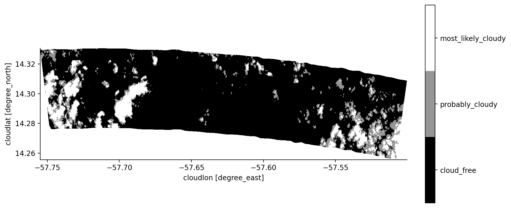
In this two-minute long sequence we can see the curvature of the HALO circle. By the way: you could also calculate the swath width of the measurements projected onto the cloud height that you specified.
Swath width#
The haversine formula is such an approximation. It calculates the great-circle distance between two points on a sphere. We just need the respective latitudes and longitudes of the points. We will use the coordinates of the two edge pixels of the first measurement.
distance_haversine_formula = haversine_distance(lat1, lat2, lon1, lon2, R = 6371)
print('The across track swath width of the measurements is about {} km'.format(np.round(distance_haversine_formula.values,2)))
The across track swath width of the measurements is about 5.95 km