Cloud radar data collected on MS Merian

General information

From here you can access the W band radar data collected on the RV MSMerian. The radar is a frequency modulated continuous-wave (FMCW) 94 GHz dual polarization radar (manufactured by RPG GmbH) and the data are published on AERIS. The data presented here are corrected for ship motions. For more details on the algorithm applied for correction, please check the paper in preparation in ESSD.

It measured continously during the campaign, with a time resolution of 3 seconds and vertical range resolution varying with height between 7.5, 9.2 and 30 m. Here we provide you with some tools to plot and visualize the data.
A quicklook browser is helping you to pick the case you are more interested in. If you have questions or if you would like to use the data for a publication, please don’t hesitate to get in contact with the dataset author that you can find here.

Getting the data catalog

The python code below allows you to browse through the days avaiable

from datetime import datetime
import matplotlib.pyplot as plt
import pathlib
plt.style.use([pathlib.Path("./mplstyle/book"), pathlib.Path("./mplstyle/wide")])
import numpy as np
import eurec4a
cat = eurec4a.get_intake_catalog(use_ipfs="QmahMN2wgPauHYkkiTGoG2TpPBmj3p5FoYJAq9uE9iXT9N")

Getting the data from the MS-Merian ship

To visualize which datasets are available for the MS-Merian ship, type:

list(cat['MS-Merian'])

['FMCW94_RPG', 'MRR_PRO', 'track']

Check available days of Wband radar data

To check which days are available from the Wband radar dataset, type:

for key, source in cat['MS-Merian']['FMCW94_RPG'].items():
    desc = source.describe()
    user_parameters = desc.get("user_parameters", [])
    if len(user_parameters) > 0:
        params = " (" + ", ".join(p["name"] for p in user_parameters) + ")"
    else:
        params = ""
    print(f"{key}{params}: {desc['description']}")
    for parameter in user_parameters:
        print(f"    {parameter['name']}: {parameter['min']} ... {parameter['max']} default: {parameter['default']}")

motion_corrected (date): daily ship motion corrected Wband radar data
    date: 2020-01-19 00:00:00 ... 2020-02-19 14:00:00 default: 2020-01-19 20:00:00

Selecting one day for plot/visualization

To work on a specific day, please provide the date as input in the form “yyyy-mm-dd hh:mm” as a field to date in the code below.

Note

The datetime type accepts multiple values: Python datetime, ISO8601 string, Unix timestamp int, “now” and “today”.

date = '2020-01-27 13:00' # <--- provide the date here 
ds = cat['MS-Merian']['FMCW94_RPG'].motion_corrected(date=date).to_dask()
ds

/usr/share/miniconda3/envs/how_to_eurec4a/lib/python3.12/site-packages/intake_xarray/base.py:21: FutureWarning: The return type of `Dataset.dims` will be changed to return a set of dimension names in future, in order to be more consistent with `DataArray.dims`. To access a mapping from dimension names to lengths, please use `Dataset.sizes`.
  'dims': dict(self._ds.dims),

<xarray.Dataset> Size: 236MB
Dimensions:                 (time: 26719, height: 550)
Coordinates:
  * height                  (height) float32 2kB 104.4 111.8 ... 9.983e+03
    lat                     (time) float32 107kB dask.array<chunksize=(26719,), meta=np.ndarray>
    lon                     (time) float32 107kB dask.array<chunksize=(26719,), meta=np.ndarray>
  * time                    (time) datetime64[ns] 214kB 2020-01-27T00:00:01 ....
Data variables: (12/13)
    air_pressure            (time) float32 107kB dask.array<chunksize=(26719,), meta=np.ndarray>
    air_temperature         (time) float32 107kB dask.array<chunksize=(26719,), meta=np.ndarray>
    brightness_temperature  (time) float32 107kB dask.array<chunksize=(26719,), meta=np.ndarray>
    instrument              <U15 60B ...
    liquid_water_path       (time) float32 107kB dask.array<chunksize=(26719,), meta=np.ndarray>
    mean_doppler_velocity   (time, height) float32 59MB dask.array<chunksize=(3340, 69), meta=np.ndarray>
    ...                      ...
    rain_rate               (time) float32 107kB dask.array<chunksize=(26719,), meta=np.ndarray>
    relative_humidity       (time) float32 107kB dask.array<chunksize=(26719,), meta=np.ndarray>
    skewness                (time, height) float32 59MB dask.array<chunksize=(3340, 69), meta=np.ndarray>
    spectral_width          (time, height) float32 59MB dask.array<chunksize=(3340, 69), meta=np.ndarray>
    wind_direction          (time) float32 107kB dask.array<chunksize=(26719,), meta=np.ndarray>
    wind_speed              (time) float32 107kB dask.array<chunksize=(26719,), meta=np.ndarray>
Attributes: (12/30)
    COMMENT:           
    CREATED_BY:        Claudia Acquistapace
    CREATED_ON:        2021-07-01 11:35:01.608208
    Conventions:       CF-1.8
    DATA_DESCRIPTION:  daily w-band radar Doppler moments and surface weather...
    DATA_DISCIPLINE:   Atmospheric Physics - Remote Sensing Radar Profiler
    ...                ...
    PI_MAIL:           cacquist@meteo.uni-koeln.de
    PI_NAME:           Claudia Acquistapace
    featureType:       trajectoryProfile
    history:           source: wband data postprocessed\nprocessing: ship mot...
    institution:       University of Cologne - Germany
    title:             daily w-band radar Doppler moments and surface weather...

xarray.Dataset

• Dimensions:
  • time: 26719
  • height: 550
• Coordinates: (4)
  • height
    (height)
    float32
    104.4 111.8 ... 9.949e+03 9.983e+03

    axis :

    Z

    long_name :

    radar_range_height

    positive :

    up

    units :

    m

    array([ 104.3517 ,  111.8054 ,  119.25909, ..., 9914.502  , 9948.572  ,
           9982.643  ], dtype=float32)

  • lat
    (time)
    float32
    dask.array<chunksize=(26719,), meta=np.ndarray>

    axis :

    Y

    standard_name :

    latitude

    units :

    degree_north

    Array Chunk Bytes 104.37 kiB 104.37 kiB Shape (26719,) (26719,) Dask graph 1 chunks in 2 graph layers Data type float32 numpy.ndarray

  • lon
    (time)
    float32
    dask.array<chunksize=(26719,), meta=np.ndarray>

    axis :

    X

    standard_name :

    longitude

    units :

    degree_east

    Array Chunk Bytes 104.37 kiB 104.37 kiB Shape (26719,) (26719,) Dask graph 1 chunks in 2 graph layers Data type float32 numpy.ndarray

  • time
    (time)
    datetime64[ns]
    2020-01-27T00:00:01 ... 2020-01-...

    axis :

    T

    standard_name :

    time

    array(['2020-01-27T00:00:01.000000000', '2020-01-27T00:00:05.000000000',
           '2020-01-27T00:00:08.000000000', ..., '2020-01-27T23:59:52.000000000',
           '2020-01-27T23:59:55.000000000', '2020-01-27T23:59:58.000000000'],
          dtype='datetime64[ns]')

• Data variables: (13)
  • air_pressure
    (time)
    float32
    dask.array<chunksize=(26719,), meta=np.ndarray>

    long_name :

    surface air pressure

    standard_name :

    surface_air_pressure

    units :

    hPa

    Array Chunk Bytes 104.37 kiB 104.37 kiB Shape (26719,) (26719,) Dask graph 1 chunks in 2 graph layers Data type float32 numpy.ndarray

  • air_temperature
    (time)
    float32
    dask.array<chunksize=(26719,), meta=np.ndarray>

    long_name :

    surface temperature

    standard_name :

    air_temperature

    units :

    degC

    Array Chunk Bytes 104.37 kiB 104.37 kiB Shape (26719,) (26719,) Dask graph 1 chunks in 2 graph layers Data type float32 numpy.ndarray

  • brightness_temperature
    (time)
    float32
    dask.array<chunksize=(26719,), meta=np.ndarray>

    long_name :

    brightness temperature at 89 GHz

    standard_name :

    brightness_temperature

    units :

    K

    Array Chunk Bytes 104.37 kiB 104.37 kiB Shape (26719,) (26719,) Dask graph 1 chunks in 2 graph layers Data type float32 numpy.ndarray

  • instrument
    ()
    <U15
    ...

    cf_role :

    trajectory_id

    [1 values with dtype=<U15]

  • liquid_water_path
    (time)
    float32
    dask.array<chunksize=(26719,), meta=np.ndarray>

    comment :

    retrieval based on neural networks developed by the manufacturer

    long_name :

    liquid water path

    standard_name :

    atmosphere_cloud_liquid_water_content

    units :

    g m-2

    Array Chunk Bytes 104.37 kiB 104.37 kiB Shape (26719,) (26719,) Dask graph 1 chunks in 2 graph layers Data type float32 numpy.ndarray

  • mean_doppler_velocity
    (time, height)
    float32
    dask.array<chunksize=(3340, 69), meta=np.ndarray>

    comment :

    mean Doppler velocity after correction for ship motions and smoothing

    long_name :

    mean Doppler velocity

    units :

    m s-1

    Array Chunk Bytes 56.06 MiB 900.23 kiB Shape (26719, 550) (3340, 69) Dask graph 64 chunks in 2 graph layers Data type float32 numpy.ndarray

  • radar_reflectivity
    (time, height)
    float32
    dask.array<chunksize=(3340, 69), meta=np.ndarray>

    long_name :

    equivalent reflectivity factor

    standard_name :

    equivalent_reflectivity_factor

    units :

    dBZ

    Array Chunk Bytes 56.06 MiB 900.23 kiB Shape (26719, 550) (3340, 69) Dask graph 64 chunks in 2 graph layers Data type float32 numpy.ndarray

  • rain_rate
    (time)
    float32
    dask.array<chunksize=(26719,), meta=np.ndarray>

    long_name :

    surface rain rate

    standard_name :

    rainfall_rate

    units :

    mm h-1

    Array Chunk Bytes 104.37 kiB 104.37 kiB Shape (26719,) (26719,) Dask graph 1 chunks in 2 graph layers Data type float32 numpy.ndarray

  • relative_humidity
    (time)
    float32
    dask.array<chunksize=(26719,), meta=np.ndarray>

    long_name :

    surface relative humidity

    standard_name :

    relative_humidity

    units :

    1

    Array Chunk Bytes 104.37 kiB 104.37 kiB Shape (26719,) (26719,) Dask graph 1 chunks in 2 graph layers Data type float32 numpy.ndarray

  • skewness
    (time, height)
    float32
    dask.array<chunksize=(3340, 69), meta=np.ndarray>

    long_name :

    skewness

    units :

    Array Chunk Bytes 56.06 MiB 900.23 kiB Shape (26719, 550) (3340, 69) Dask graph 64 chunks in 2 graph layers Data type float32 numpy.ndarray

  • spectral_width
    (time, height)
    float32
    dask.array<chunksize=(3340, 69), meta=np.ndarray>

    long_name :

    spectral width

    units :

    m s-1

    Array Chunk Bytes 56.06 MiB 900.23 kiB Shape (26719, 550) (3340, 69) Dask graph 64 chunks in 2 graph layers Data type float32 numpy.ndarray

  • wind_direction
    (time)
    float32
    dask.array<chunksize=(26719,), meta=np.ndarray>

    long_name :

    surface wind direction

    standard_name :

    wind_from_direction

    units :

    degrees

    Array Chunk Bytes 104.37 kiB 104.37 kiB Shape (26719,) (26719,) Dask graph 1 chunks in 2 graph layers Data type float32 numpy.ndarray

  • wind_speed
    (time)
    float32
    dask.array<chunksize=(26719,), meta=np.ndarray>

    long_name :

    surface horizontal wind speed

    standard_name :

    wind_speed

    units :

    m s-1

    Array Chunk Bytes 104.37 kiB 104.37 kiB Shape (26719,) (26719,) Dask graph 1 chunks in 2 graph layers Data type float32 numpy.ndarray

• Indexes: (2)
  • height
    PandasIndex

    PandasIndex(Index([104.35169982910156,  111.8053970336914, 119.25908660888672,
           126.71277618408203, 134.16647338867188,  141.6201629638672,
            149.0738525390625, 156.52755737304688,  163.9812469482422,
            171.4349365234375,
           ...
              9676.0087890625,    9710.0791015625,    9744.1494140625,
              9778.2197265625,     9812.291015625,     9846.361328125,
               9880.431640625,     9914.501953125,     9948.572265625,
               9982.642578125],
          dtype='float32', name='height', length=550))

  • time
    PandasIndex

    PandasIndex(DatetimeIndex(['2020-01-27 00:00:01', '2020-01-27 00:00:05',
                   '2020-01-27 00:00:08', '2020-01-27 00:00:11',
                   '2020-01-27 00:00:14', '2020-01-27 00:00:17',
                   '2020-01-27 00:00:21', '2020-01-27 00:00:24',
                   '2020-01-27 00:00:27', '2020-01-27 00:00:30',
                   ...
                   '2020-01-27 23:59:29', '2020-01-27 23:59:32',
                   '2020-01-27 23:59:36', '2020-01-27 23:59:39',
                   '2020-01-27 23:59:42', '2020-01-27 23:59:45',
                   '2020-01-27 23:59:48', '2020-01-27 23:59:52',
                   '2020-01-27 23:59:55', '2020-01-27 23:59:58'],
                  dtype='datetime64[ns]', name='time', length=26719, freq=None))

• Attributes: (30)

  COMMENT :

  CREATED_BY :

  Claudia Acquistapace

  CREATED_ON :

  2021-07-01 11:35:01.608208

  Conventions :

  CF-1.8

  DATA_DESCRIPTION :

  daily w-band radar Doppler moments and surface weather station variables

  DATA_DISCIPLINE :

  Atmospheric Physics - Remote Sensing Radar Profiler

  DATA_GROUP :

  Experimental;Profile;Moving

  DATA_LOCATION :

  Research vessel Maria S. Merian - Atlantic Ocean

  DATA_PROCESSING :

  ship motion correction, the code used is available at https://github.com/ClauClouds/ship-motion-correction-for-EUREC4A-campaign

  DATA_SOURCE :

  wband data postprocessed

  DOI :

  10.25326/235 (https://doi.org/10.25326/235)

  DO_AFFILIATION :

  University of Cologne - Germany

  DO_MAIL :

  cacquist@meteo.uni-koeln.de

  DO_NAME :

  University of Cologne - Germany

  DO_address :

  Institute for geophysics and meteorology, Pohligstrasse 3, 50696 Koeln

  DS_AFFILIATION :

  University of Cologne - Germany

  DS_MAIL :

  cacquist@meteo.uni-koeln.de

  DS_NAME :

  University of Cologne - Germany

  DS_address :

  Institute for geophysics and meteorology, Pohligstrasse 3, 50696 Koeln

  FILL_VALUE :

  NaN

  INSTRUMENT_MODEL :

  94 GHz (W-band) radar, manufactured by RPG GmbH

  ORCID-AUTHOR :

  Claudia Acquistapace: 0000-0002-1144-4753

  PI_ADDRESS :

  Institute for geophysics and meteorology, Pohligstrasse 3, 50969 Koeln

  PI_AFFILIATION :

  University of Cologne (UNI), Germany

  PI_MAIL :

  cacquist@meteo.uni-koeln.de

  PI_NAME :

  Claudia Acquistapace

  featureType :

  trajectoryProfile

  history :

  source: wband data postprocessed processing: ship motion correction, the code used is available at https://github.com/ClauClouds/ship-motion-correction-for-EUREC4A-campaign adapted to enhance CF compatibility

  institution :

  University of Cologne - Germany

  title :

  daily w-band radar Doppler moments and surface weather station variables

Plot some radar quantities

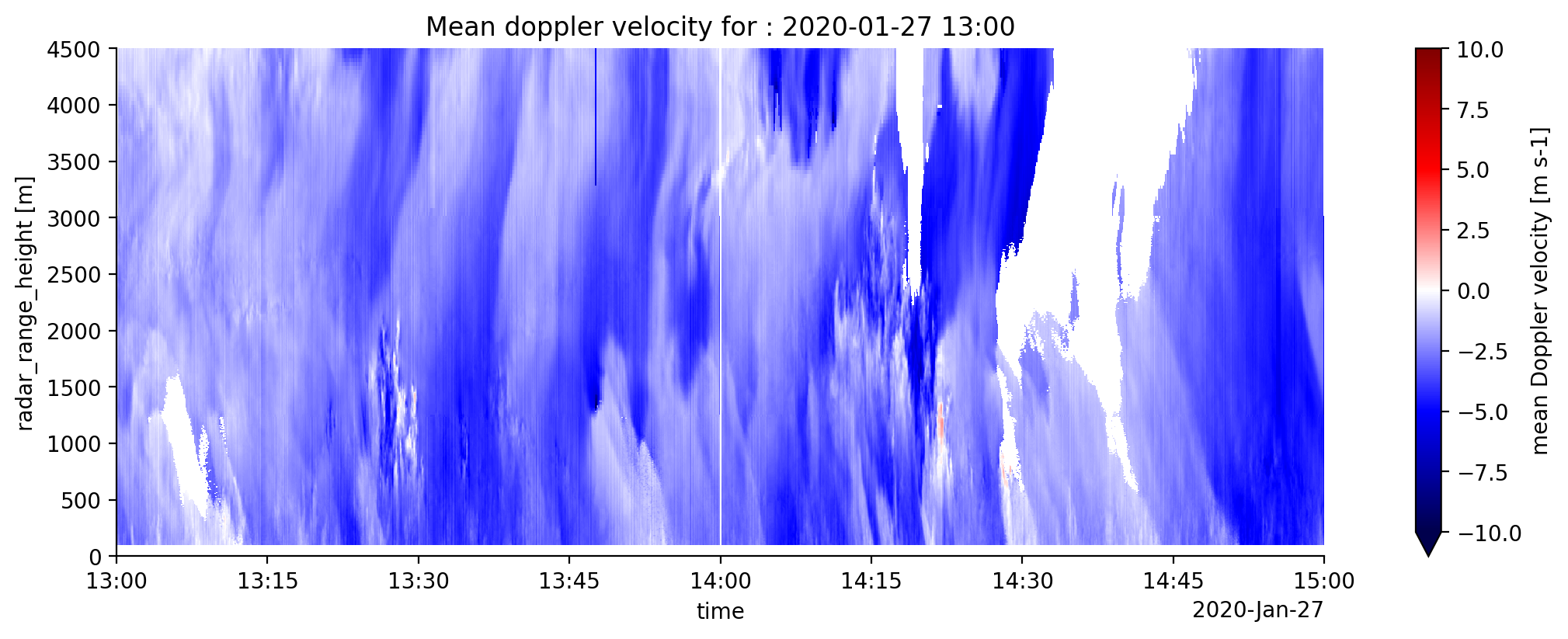
To create time/height plots for radar moments, pick a variable name having dimension (time, height) from the list of data variables and type the name in the code below. The example here is for mean Doppler velocity (corrected for ship motions). You can decide to either select the entire day or a given hour by providing time_min and time_max. To provide time_min and time_max, modify the string ‘yyyy-mm-ddThh:mm:ss’ Example: to select the entire day :

time_min = np.datetime64('2020-01-27T00:00:00')
time_max = np.datetime64('2020-01-27T23:59:59')

to select between 13:00 and 15:00 UTC:

time_min = np.datetime64('2020-01-27T13:00:00')
time_max = np.datetime64('2020-01-27T15:00:00')

# set min and max time values for plotting along the x-axis
time_min = np.datetime64('2020-01-27T13:00:00') # insert the string value corresponding to t_min
time_max = np.datetime64('2020-01-27T15:00:00') # insert the string value corresponding to t_max

# selecting subset of data
ds_sliced = ds.sel(time=slice(time_min, time_max))

fig, ax = plt.subplots()
# set here the variable from ds to plot, its color map and its min and max values
ds_sliced.mean_doppler_velocity.plot(x='time', y='height', cmap="seismic", vmin=-10., vmax=10.)
ax.set_title("Mean doppler velocity for : "+date)
ax.set_xlim(time_min, time_max)
ax.set_ylim(0, 4500);

Check corresponding merian position in the selected hour

We use the function track2layer defined in the interactive HALO tracks chapter, and we provide as input the data for the time interval selected during the day

import ipyleaflet

# function to associate features to a given track
def track2layer(track, color="green", name=""):
    return ipyleaflet.Polyline(
        locations=np.stack([track.lat.values, track.lon.values], axis=1).tolist(), 
        color=color,
        fill=True,
        weight=4,
        name=name
    )

# definition of the base map 
m = ipyleaflet.Map(
    basemap=ipyleaflet.basemaps.Esri.NatGeoWorldMap,
    center=(11.3, -57), zoom=6)
m.add_layer(track2layer(ds_sliced, 'red', 'merian position'))  # adding layer of merian position
m.add_control(ipyleaflet.ScaleControl(position='bottomleft'))
m.add_control(ipyleaflet.LayersControl(position='topright'))
m.add_control(ipyleaflet.FullScreenControl())
display(m)