BACARDI dataset

The following script exemplifies the access and usage of the Broadband AirCrAft RaDiometer Instrumentation (BACARDI), that combines two sets of Kipp and Zonen broadband radiometer measuring upward and downward irradiance in the solar (pyranometer model CMP-22, 0.2 - 3.6 μm) and terrestrial (pyrgeometer model CGR-4, 4.5 - 42 μm) spectral range.

The dataset is published under Ehrlich et al. (2021). If you have questions or if you would like to use the data for a publication, please don’t hesitate to get in contact with the dataset authors as stated in the dataset attributes contact or author.

Get data

• To load the data we first load the EUREC⁴A meta data catalogue. More information on the catalog can be found here.

import eurec4a

cat = eurec4a.get_intake_catalog(use_ipfs="QmahMN2wgPauHYkkiTGoG2TpPBmj3p5FoYJAq9uE9iXT9N")
list(cat.HALO.BACARDI)

['irradiances']

• We can further specify the platform, instrument, if applicable dataset level or variable name, and pass it on to dask.

Note

Have a look at the attributes of the xarray dataset ds for all relevant information on the dataset, such as author, contact, or citation infromation.

ds = cat.HALO.BACARDI.irradiances['HALO-0205'].to_dask()
ds

/usr/share/miniconda3/envs/how_to_eurec4a/lib/python3.12/site-packages/intake_xarray/base.py:21: FutureWarning: The return type of `Dataset.dims` will be changed to return a set of dimension names in future, in order to be more consistent with `DataArray.dims`. To access a mapping from dimension names to lengths, please use `Dataset.sizes`.
  'dims': dict(self._ds.dims),

<xarray.Dataset> Size: 17MB
Dimensions:             (time: 327320)
Coordinates:
  * time                (time) datetime64[ns] 3MB 2020-02-05T09:15:52 ... 202...
Data variables:
    F_down_solar        (time) float32 1MB dask.array<chunksize=(81830,), meta=np.ndarray>
    F_down_solar_diff   (time) float32 1MB dask.array<chunksize=(81830,), meta=np.ndarray>
    F_down_solar_sim    (time) float32 1MB dask.array<chunksize=(81830,), meta=np.ndarray>
    F_down_terrestrial  (time) float32 1MB dask.array<chunksize=(81830,), meta=np.ndarray>
    F_up_solar          (time) float32 1MB dask.array<chunksize=(81830,), meta=np.ndarray>
    F_up_terrestrial    (time) float32 1MB dask.array<chunksize=(81830,), meta=np.ndarray>
    alt                 (time) float32 1MB dask.array<chunksize=(81830,), meta=np.ndarray>
    cloud_mask          (time) int8 327kB dask.array<chunksize=(163660,), meta=np.ndarray>
    lat                 (time) float32 1MB dask.array<chunksize=(81830,), meta=np.ndarray>
    lon                 (time) float32 1MB dask.array<chunksize=(81830,), meta=np.ndarray>
    saa                 (time) float32 1MB dask.array<chunksize=(81830,), meta=np.ndarray>
    sza                 (time) float32 1MB dask.array<chunksize=(81830,), meta=np.ndarray>
Attributes:
    campaign:             EUREC4A
    comment 1:            BACARDI Raw data was processed by DLR, contact Andr...
    contact:              Andre Ehrlich, University Leipzig, a.ehrlich@uni-le...
    instrument:           Broadband AirCrAft RaDiometer Instrumentation (BACA...
    platform:             HALO
    research_flight_day:  2020/02/05
    title:                Broadband radiation mesured by BACARDI during EUREC4A
    version:              Revision 1 from 2021/02/04

xarray.Dataset

• Dimensions:
  • time: 327320
• Coordinates: (1)
  • time
    (time)
    datetime64[ns]
    2020-02-05T09:15:52 ... 2020-02-...

    long_name :

    time

    array(['2020-02-05T09:15:52.000000000', '2020-02-05T09:15:52.100000000',
           '2020-02-05T09:15:52.200000000', ..., '2020-02-05T18:21:23.700000000',
           '2020-02-05T18:21:23.800000000', '2020-02-05T18:21:23.900000000'],
          dtype='datetime64[ns]')

• Data variables: (12)
  • F_down_solar
    (time)
    float32
    dask.array<chunksize=(81830,), meta=np.ndarray>

    comment1 :

    Corrected for temperature offset, time response, aircraft attitude

    comment2 :

    Temperature offset correction based on DLR parametrization

    comment3 :

    Time response correction: response time 1.2s, cut-off_frequency 0.6Hz, running mean length = 0.5s

    comment4 :

    Attitude correction: roll offset = +0.3� , pitch offset = +2.55�

    long_name :

    Downward solar irradiance corrected for cloud-free conditions (0.2-3.6 um) (BACARDI)

    standard_name :

    downwelling_shortwave_flux_in_air

    units :

    W m-2

    Array Chunk Bytes 1.25 MiB 319.65 kiB Shape (327320,) (81830,) Dask graph 4 chunks in 2 graph layers Data type float32 numpy.ndarray

  • F_down_solar_diff
    (time)
    float32
    dask.array<chunksize=(81830,), meta=np.ndarray>

    comment1 :

    Corrected for temperature offset, time response, aircraft attitude

    comment2 :

    Temperature offset correction based on DLR parametrization

    comment3 :

    Time response correction: response time 1.2s, cut-off_frequency 0.6Hz, running mean length = 0.5s

    comment4 :

    No attitude correction applied, assuming a 100% diffuse radiation field due to clouds

    long_name :

    Downward solar irradiance corrected for diffuse/cloudy conditions (0.2-3.6 um) (BACARDI)

    standard_name :

    diffuse_downwelling_shortwave_flux_in_air

    units :

    W m-2

    Array Chunk Bytes 1.25 MiB 319.65 kiB Shape (327320,) (81830,) Dask graph 4 chunks in 2 graph layers Data type float32 numpy.ndarray

  • F_down_solar_sim
    (time)
    float32
    dask.array<chunksize=(81830,), meta=np.ndarray>

    comment :

    Simulated for aircraft position, altitude using the BCO radio soundings

    long_name :

    Downward solar irradiance simulated for cloud-free conditions (with libRadtran)

    units :

    W m-2

    Array Chunk Bytes 1.25 MiB 319.65 kiB Shape (327320,) (81830,) Dask graph 4 chunks in 2 graph layers Data type float32 numpy.ndarray

  • F_down_terrestrial
    (time)
    float32
    dask.array<chunksize=(81830,), meta=np.ndarray>

    comment1 :

    Corrected for temperature offset, time response

    comment2 :

    Temperature offset correction based on DLR parametrization

    comment3 :

    Time response correction: response time 2.0s, cut-off_frequency 0.5Hz, running mean length = 2.0s

    long_name :

    Downward terrestrial irradiance (4.5-42 um) (BACARDI)

    standard_name :

    downwelling_longwave_flux_in_air

    units :

    W m-2

    Array Chunk Bytes 1.25 MiB 319.65 kiB Shape (327320,) (81830,) Dask graph 4 chunks in 2 graph layers Data type float32 numpy.ndarray

  • F_up_solar
    (time)
    float32
    dask.array<chunksize=(81830,), meta=np.ndarray>

    comment1 :

    Corrected for temperature offset, time response

    comment2 :

    Temperature offset correction based on DLR parametrization

    comment3 :

    Time response correction: response time 1.2s, cut-off_frequency 0.6Hz, running mean length = 0.5s

    long_name :

    Upward solar irradiance (0.2-3.6 um) (BACARDI)

    standard_name :

    upwelling_shortwave_flux_in_air

    units :

    W m-2

    Array Chunk Bytes 1.25 MiB 319.65 kiB Shape (327320,) (81830,) Dask graph 4 chunks in 2 graph layers Data type float32 numpy.ndarray

  • F_up_terrestrial
    (time)
    float32
    dask.array<chunksize=(81830,), meta=np.ndarray>

    comment1 :

    Corrected for temperature offset, time response

    comment2 :

    Temperature offset correction based on DLR parametrization

    comment3 :

    Time response correction: response time 2.0s, cut-off_frequency 0.5Hz, running mean length = 2.0s

    long_name :

    Upward terrestrial irradiance (4.5-42 um) (BACARDI)

    standard_name :

    upwelling_longwave_flux_in_air

    units :

    W m-2

    Array Chunk Bytes 1.25 MiB 319.65 kiB Shape (327320,) (81830,) Dask graph 4 chunks in 2 graph layers Data type float32 numpy.ndarray

  • alt
    (time)
    float32
    dask.array<chunksize=(81830,), meta=np.ndarray>

    long_name :

    altitude (WGS84 Datum/Elliptical, BAHAMAS)

    standard_name :

    altitude

    units :

    m

    Array Chunk Bytes 1.25 MiB 319.65 kiB Shape (327320,) (81830,) Dask graph 4 chunks in 2 graph layers Data type float32 numpy.ndarray

  • cloud_mask
    (time)
    int8
    dask.array<chunksize=(163660,), meta=np.ndarray>

    comment1 :

    The cloud flag is a rough conservative estimate of the presence of clouds based on the variability of the downward solar irradiance within a 20 second running window.

    long_name :

    Cloud flag for clouds in front of the Sun affecting the solar downward irradiance [0 = cloud free, 1 = cloudy]

    Array Chunk Bytes 319.65 kiB 159.82 kiB Shape (327320,) (163660,) Dask graph 2 chunks in 2 graph layers Data type int8 numpy.ndarray

  • lat
    (time)
    float32
    dask.array<chunksize=(81830,), meta=np.ndarray>

    long_name :

    latitude (WGS84 Datum/Latitude, BAHAMAS)

    standard_name :

    latitude

    units :

    degrees_north

    Array Chunk Bytes 1.25 MiB 319.65 kiB Shape (327320,) (81830,) Dask graph 4 chunks in 2 graph layers Data type float32 numpy.ndarray

  • lon
    (time)
    float32
    dask.array<chunksize=(81830,), meta=np.ndarray>

    long_name :

    longitude (WGS84 Datum/Longitude, BAHAMAS)

    standard_name :

    longitude

    units :

    degree_east

    Array Chunk Bytes 1.25 MiB 319.65 kiB Shape (327320,) (81830,) Dask graph 4 chunks in 2 graph layers Data type float32 numpy.ndarray

  • saa
    (time)
    float32
    dask.array<chunksize=(81830,), meta=np.ndarray>

    long_name :

    solar azimuth angle

    standard_name :

    solar_azimuth_angle

    units :

    degree

    Array Chunk Bytes 1.25 MiB 319.65 kiB Shape (327320,) (81830,) Dask graph 4 chunks in 2 graph layers Data type float32 numpy.ndarray

  • sza
    (time)
    float32
    dask.array<chunksize=(81830,), meta=np.ndarray>

    long_name :

    solar zenith angle

    standard_name :

    solar_zenith_angle

    units :

    degree

    Array Chunk Bytes 1.25 MiB 319.65 kiB Shape (327320,) (81830,) Dask graph 4 chunks in 2 graph layers Data type float32 numpy.ndarray

• Indexes: (1)
  • time
    PandasIndex

    PandasIndex(DatetimeIndex([       '2020-02-05 09:15:52', '2020-02-05 09:15:52.100000',
                   '2020-02-05 09:15:52.200000', '2020-02-05 09:15:52.300000',
                   '2020-02-05 09:15:52.400000', '2020-02-05 09:15:52.500000',
                   '2020-02-05 09:15:52.600000', '2020-02-05 09:15:52.700000',
                   '2020-02-05 09:15:52.800000', '2020-02-05 09:15:52.900000',
                   ...
                          '2020-02-05 18:21:23', '2020-02-05 18:21:23.100000',
                   '2020-02-05 18:21:23.200000', '2020-02-05 18:21:23.300000',
                   '2020-02-05 18:21:23.400000', '2020-02-05 18:21:23.500000',
                   '2020-02-05 18:21:23.600000', '2020-02-05 18:21:23.700000',
                   '2020-02-05 18:21:23.800000', '2020-02-05 18:21:23.900000'],
                  dtype='datetime64[ns]', name='time', length=327320, freq=None))

• Attributes: (8)

  campaign :

  EUREC4A

  comment 1 :

  BACARDI Raw data was processed by DLR, contact Andreas Giez

  contact :

  Andre Ehrlich, University Leipzig, a.ehrlich@uni-leipzig.de

  instrument :

  Broadband AirCrAft RaDiometer Instrumentation (BACARDI)

  platform :

  HALO

  research_flight_day :

  2020/02/05

  title :

  Broadband radiation mesured by BACARDI during EUREC4A

  version :

  Revision 1 from 2021/02/04

The data from EUREC⁴A is of 10 Hz measurement frequency and corrected for dynamic temperature effects. For the downward solar irradiance, data are provided with and without aircraft attitude correction corresponding to cloud-free and cloudy conditions, respectively, above HALO.

Plots

We plot the upward and downward irradiances in two panels.

%matplotlib inline
import pathlib
import matplotlib.pyplot as plt
plt.style.use([pathlib.Path("./mplstyle/book"), pathlib.Path("./mplstyle/wide")])

fig, (ax1, ax2) = plt.subplots(1, 2)
ax1.set_prop_cycle(color=['darkblue', 'red'])
for var in ['F_up_solar', 'F_up_terrestrial']:
    ds[var].plot(ax=ax1,label= var)
ax1.legend()
ax1.set_ylabel('upward solar and terrestrial irradiance / Wm$^{-2}$')

ax2.set_prop_cycle(color=['grey', 'skyblue', 'darkblue'])
for var in ['F_down_solar_sim', 'F_down_solar_diff', 'F_down_solar']:
    ds[var].plot(ax=ax2, label= var)
ax2.legend()
ax2.set_ylabel('downward solar irradiance / Wm$^{-2}$');

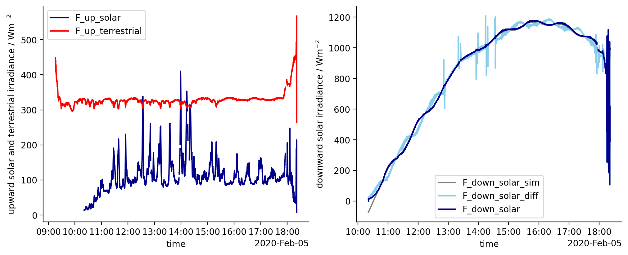
The attitude correction of downward solar irradiance does not account for the present cloud situation above HALO. Instead, two data sets, one assuming cloud-free and one assuming overcast (diffuse illumination) conditions, are provided. Depending on the application, the user needs to choose between both data sets. For the downward solar irradiance assuming cloud-free conditions, the data are filtered for turns of HALO, high roll and pitch angles. This filter is not applied for the data assuming overcast/diffuse conditions to provide the full data. However, data during turns of HALO need to be analysed with care. As shown in the example some artifical spikes due to turns are present in the data.

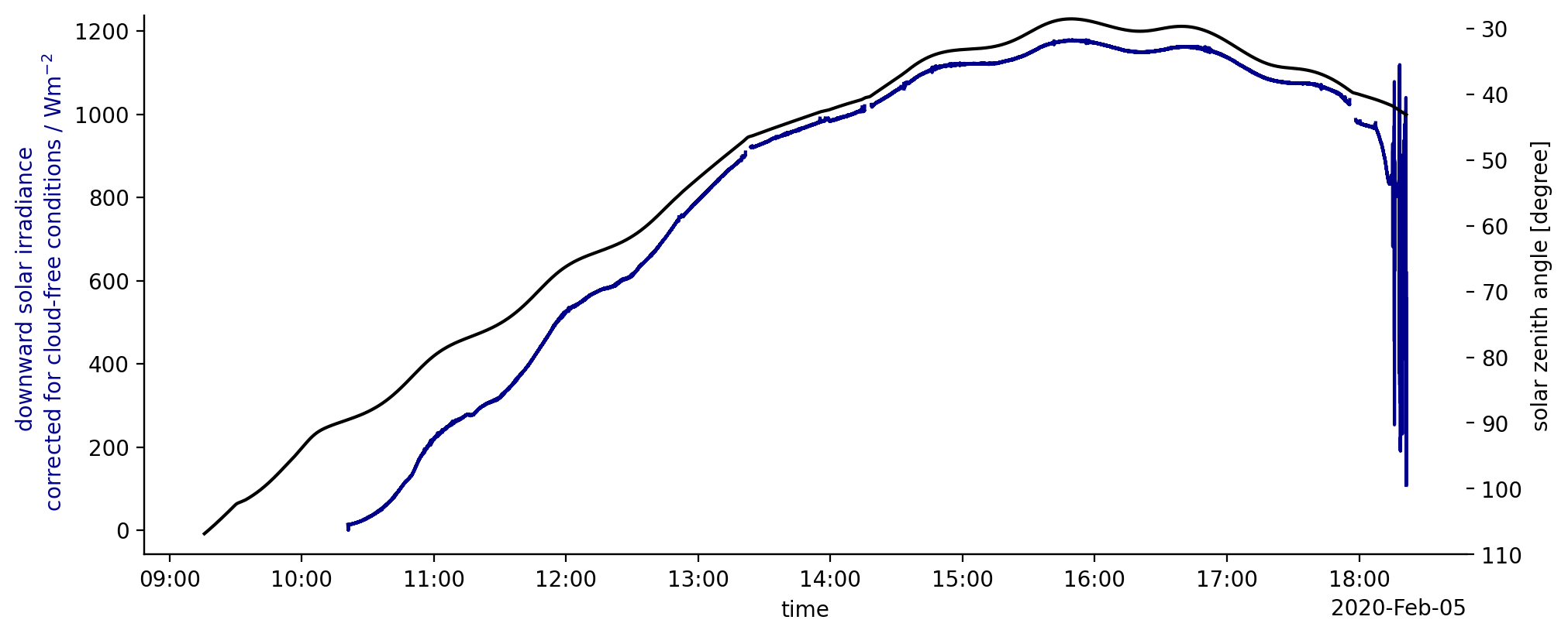
The wiggles originate from the about 200km change in location and therewith solar zenith angle within one circle / hour as can be seen in a plot.

fig, ax = plt.subplots()
ds.F_down_solar.plot(ax=ax, color='darkblue')
ax.set_ylabel('downward solar irradiance \n corrected for cloud-free conditions / Wm$^{-2}$',
              color='darkblue')
ax2 = ax.twinx()
ds.sza.plot(ax=ax2, color='black')
ax2.set_ylim(110, 28);