specMACS cloud geometry

specMACS cloud geometry#

In the following, an example of how to use the specMACS cloud geometry dataset will be shown. The cloud geometry is retrieved by a stereographic feature matching method described by Kölling et al. (2019). The algorithm is applied to the data of the two polarization resolving cameras of the instrument covering a large combined field of view of about \(\pm 45° \times \pm 59°\) (along track \(\times\) across track) (Pörtge et al., 2023). It is important to mention that no points found does not necessarily mean that no cloud has been observed as this can also happen if the cloud lacks in contrasts or due to a bad tracking of features.

Simple plots#

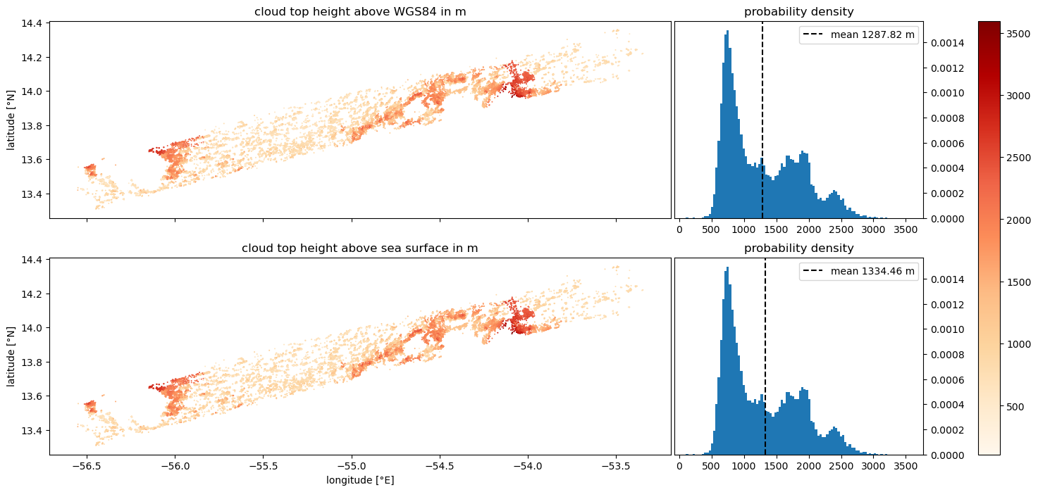
We will start to do some first simple scatter plots of the cloud top heights (CTH). There are two CTH variables in the dataset: A normal ‘height’ variable and a variable called ‘height_above_geoid’. The first is defined with respect to the WGS84 ellipsoid and the second with respect to the EGM2008 geoid. Although there is not a large difference between both in the EUREC4A area, we will exemplarily plot both.

import numpy as np
import matplotlib.pyplot as plt
from mpl_toolkits.axes_grid1 import make_axes_locatable

We’ll select only every 100th data point for a quick overview.

Important

Depending on the clouds there might be a lot of points in the dataset or not such that this step might be useful or not.

ds_sel = ds.isel(sample=slice(0, None, 100))

load the data variables

lat = ds_sel['lat'].values
lon = ds_sel['lon'].values
height = ds_sel['height'].values
height_above_geoid = ds_sel['height_above_geoid'].values

cmap = 'OrRd'
vmin = np.min([height, height_above_geoid])
vmax = np.max([height, height_above_geoid])

fig, axs = plt.subplots(nrows=2, ncols=1, figsize=(20, 8), sharex=True)
for ax, var, ref in zip(axs, [height, height_above_geoid], ["WGS84", "sea surface"]):
    sm = ax.scatter(lon, lat, c=var, marker='o', s=2, edgecolor=None, linewidth=0, vmin=vmin, vmax=vmax, cmap=cmap)
    ax.set_title(f'cloud top height above {ref} in m')
    ax.set_ylabel('latitude [°N]')
    divider = make_axes_locatable(ax)
    ax2 = divider.append_axes('right', size='40%', pad=0.05)
    ax2.hist(height, bins=100, range=(vmin, vmax), density=True)
    ax2.set_title('probability density')
    ax2.yaxis.tick_right()
    ax2.axvline(np.mean(var), linestyle='dashed', color='k', label='mean {:.2f} m'.format(np.mean(var)))
    ax2.legend()

axs[1].set_xlabel('longitude [°E]')
plt.colorbar(sm, ax=axs)
None

_images/283efb9376320bf69f37c33ff1ce0436013cfaf104f7b190aabeb924273e73d4.png

Make a 3D plot#

As the stereo points are points on the cloud surface located in 3D space, we can also do a 3D plot. We will use a few different viewing settings, which can also be individually adjusted using the elev and azim arguments of the ax.view_init setting.

import matplotlib.ticker as ticker

settings for plots

markersize = 0.1
cmap = 'viridis' #colormap
vmin = np.min(height)
vmax = np.max(height)

fig, axs = plt.subplots(2, 2, figsize=(14,12), subplot_kw=dict(projection='3d'))

for ax in axs.ravel():
    sm = ax.scatter(lon, lat, height, c=height, marker='o', vmin=vmin, vmax=vmax, cmap=cmap, s=markersize, linewidths=None, edgecolors=None)

ax = axs[0,0]
ax.set_xlabel('longitude [°E]', labelpad=6.0)
ax.set_ylabel('latitude [°N]', labelpad=6.0)
ax.set_zlabel('height above WGS84 [m]', labelpad=6.0)
ax.view_init(elev=None, azim=None)
ax.set_title('3D stereo plot', y=1.02)

ax = axs[0,1]
ax.set_ylabel('latitude [°N]', labelpad=6.0)
ax.set_zlabel('height above WGS84 [m]', labelpad=6.0)
ax.view_init(elev=0, azim=0)
ax.set_title('latitude-height plane', y=1.02)
ax.xaxis.set_major_locator(ticker.NullLocator())

ax = axs[1,0]
ax.set_xlabel('longitude [°E]', labelpad=4.0)
ax.set_ylabel('latitude [°N]', labelpad=6.0)
ax.view_init(elev=90, azim=-90)
ax.set_title('longitude-latitude plane', y=1.02)
ax.zaxis.set_major_locator(ticker.NullLocator())

ax = axs[1,1]
ax.set_xlabel('longitude [°E]', labelpad=6.0)
ax.set_zlabel('height above WGS84 [m]', labelpad=10.0)
ax.view_init(elev=0, azim=-90)
ax.set_title('longitude-height plane', y=1.02)
ax.yaxis.set_major_locator(ticker.NullLocator())

plt.subplots_adjust(bottom=0.1, right=0.9)
cax = plt.axes([0.95, 0.15, 0.05, 0.7])
fig.colorbar(sm, cax=cax, label='height above WGS84 [m]', fraction=0.02, shrink=2.0, aspect=40)
None

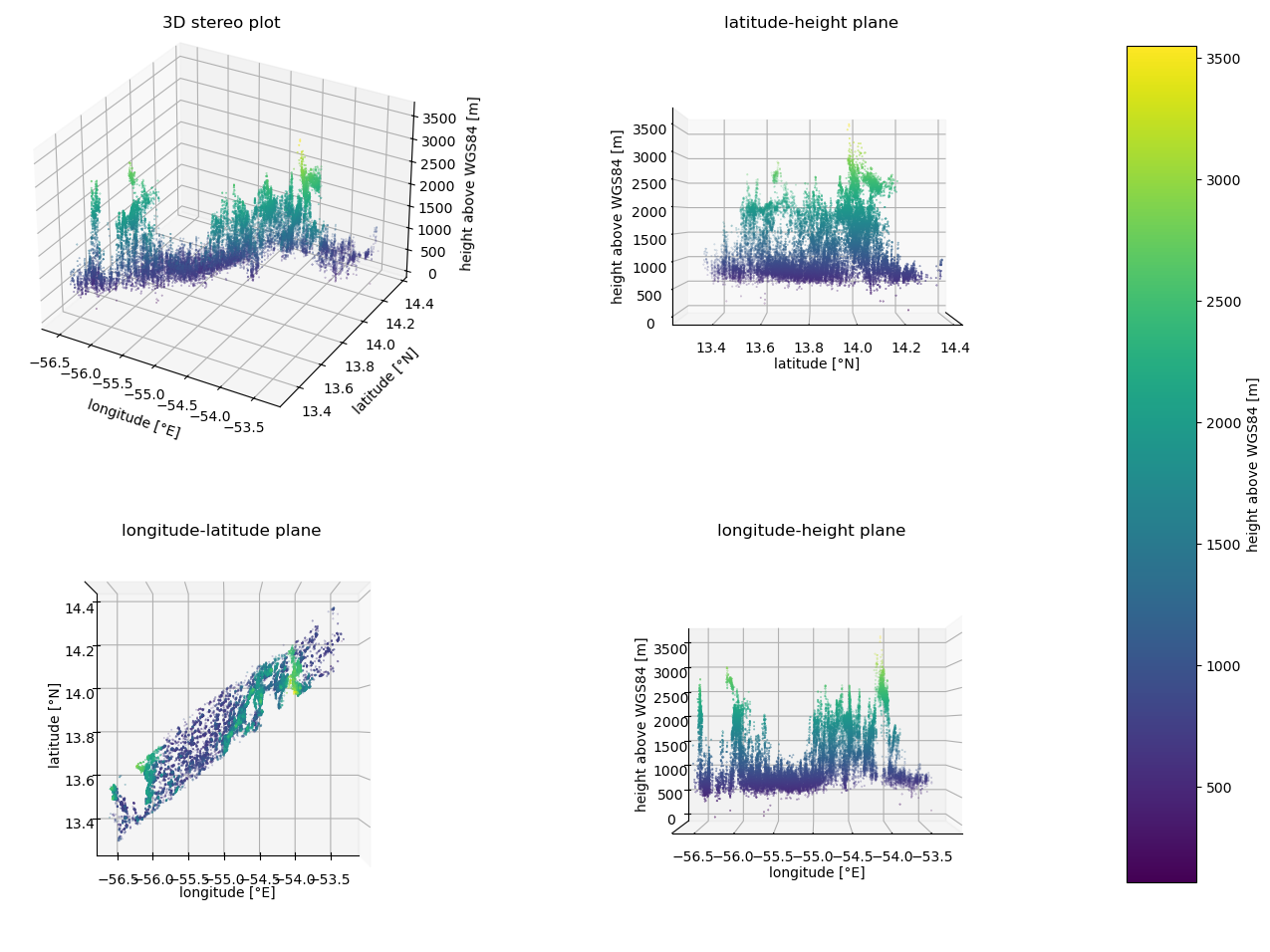
_images/35938020ca2d0c517d463363811c404b013baf8a0f386590e6b559221c7414c3.png

The 3D plots show the scene from different perspectives. It can be seen that the tracking algorithm finds points in both cloud layers down to a base height of approximately 1000m. Below, there are also some points which are probably outliers due to some wrong identifications.

Project points to specMACS measurements#

We will start to project the points found from the stereographic reconstruction to pre-rendered specMACS tile maps which can be found here. To make them available to cartopy, we need a little helper class specMACSPTiles, which mainly takes care of making unavailable tiles transparent (these are outside the viewing range of the instrument).

We can now get the tile map for our selected flight segment:

specmacs = specMACSPTiles(segment_id)

Get vmin and vmax using quantiles such that outliers will not influence the colorbar too much:

q = 0.01
vmin, vmax = np.quantile(height, [q, 1-q])
cmap = 'OrRd'

import cartopy.crs as ccrs

fig, axes = plt.subplots(1, 2, figsize=(16, 8), constrained_layout=True, subplot_kw={"projection": ccrs.PlateCarree()})
for ax in axes:
    ax.set_extent([np.floor(np.min(lon)), np.ceil(np.max(lon)), np.floor(np.min(lat)), np.ceil(np.max(lat))], crs=ccrs.PlateCarree())
    ax.add_image(specmacs, 8)  # the number is an integer and represents the detail level. It is logarithmic, small values are coarse, large values are fine.
    ax.set_axis_off()
im = ax.scatter(lon, lat, c=height, marker="o", s=0.4, edgecolor=None, linewidth=0, vmin=vmin, vmax=vmax, cmap=cmap)
fig.colorbar(im, label='height above WGS84 [m]', extend='both', shrink=0.4)
None

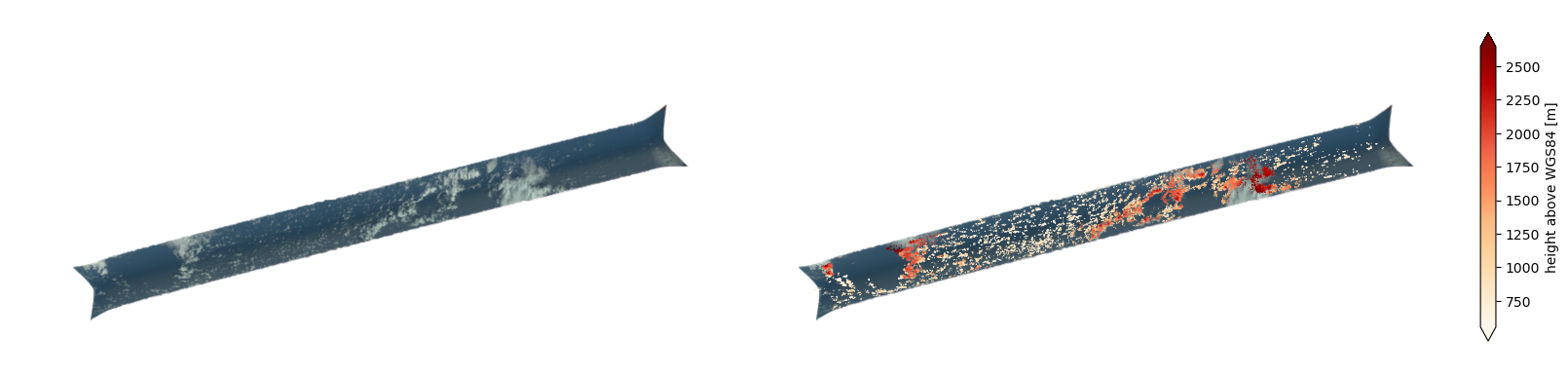
_images/12d71182adb1b4ab37e274d81ac971ac9b35d54e1a12c789b48c3da8c8ee2d9c.png

The projection of the points to the specMACS map on the right shows that most of the clouds, in particular the small cumulus clouds are well identified and located by the stereographic reconstruction method. The only exception is the higher and thicker cloud toward the end of the leg. This cloud lacks contrasts such that only its edges are identified well by the tracking algorithm.

specMACS cloud geometry

Contents

specMACS cloud geometry#

Open dataset#

Simple plots#

Make a 3D plot#

Project points to specMACS measurements#