W-band radar example

During EUREC⁴A and ATOMIC NOAA deployed W-band (94 GHz) radars on both the P-3 aircraft and the ship Ron Brown. The airborne radar was operated with 220 30-meter range gates with a dwell time of 0.5 seconds. The minimum detectable reflectivity of -36 dBZ at a range of 1 km although accurate estimates of Doppler properties require about -30 dBZ at 1 km.

The data are available through the EUREC⁴A intake catalog.

import datetime

import matplotlib.pyplot as plt
import colorcet as cc
%matplotlib inline

import eurec4a
cat = eurec4a.get_intake_catalog(use_ipfs="QmahMN2wgPauHYkkiTGoG2TpPBmj3p5FoYJAq9uE9iXT9N")

We’ll select an hour’s worth of observations from a single flight day, and mask out any observations with signal-to-noise ratio less than -10 dB.

time_slice = slice(datetime.datetime(2020, 1, 19, hour=18),
                   datetime.datetime(2020, 1, 19, hour=19))

cloud_params = cat.P3.remote_sensing['P3-0119'].to_dask().sel(time=time_slice)

w_band         = cat.P3.w_band_radar['P3-0119'].to_dask().sel(time=time_slice, height=slice(0,3))
w_band         = w_band.where(w_band.snr > -10)

/usr/share/miniconda3/envs/how_to_eurec4a/lib/python3.12/site-packages/intake_xarray/base.py:21: FutureWarning: The return type of `Dataset.dims` will be changed to return a set of dimension names in future, in order to be more consistent with `DataArray.dims`. To access a mapping from dimension names to lengths, please use `Dataset.sizes`.
  'dims': dict(self._ds.dims),

/usr/share/miniconda3/envs/how_to_eurec4a/lib/python3.12/site-packages/intake_xarray/base.py:21: FutureWarning: The return type of `Dataset.dims` will be changed to return a set of dimension names in future, in order to be more consistent with `DataArray.dims`. To access a mapping from dimension names to lengths, please use `Dataset.sizes`.
  'dims': dict(self._ds.dims),

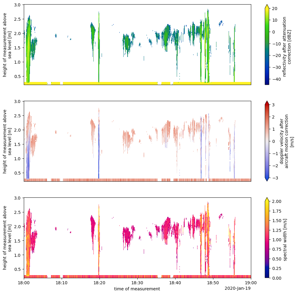
The three main quantities measured by the radar are the reflectivity, the Doppler velocity, and the spectral width.

fig = plt.figure(figsize = (12,10.2))

axes = fig.subplots(3, 1, sharex=True)
w_band.corrected_reflectivity.plot(x="time", y="height",
                                   ax = axes[0],
                                   vmin = -45, vmax = 20,
                                   cmap = cc.m_bgy)
w_band.corrected_doppler_velocity.plot(x="time", y="height",
                                       ax = axes[1],
                                       vmin = -3, vmax = 3,
                                       cmap = cc.m_coolwarm)

w_band.spectral_width.plot(x="time", y="height",
                          ax = axes[2],
                          vmin = 0, vmax = 2,
                          cmap = cc.m_bmy)

for ax in axes[0:2]:
    ax.tick_params(
    axis='x',          # changes apply to the x-axis
    which='both',      # both major and minor ticks are affected
    bottom=False,      # ticks along the bottom edge are off
    top=False,         # ticks along the top edge are off
    labelbottom=False) # labels along the bottom edge are off
    ax.xaxis.set_visible(False)

fig.subplots_adjust(bottom = 0)